Mulling over matrix multiplications in CUDA

\[\require{amsmath}\]

This post is about some details I find useful to keep in mind when optimizing performance of machine learning models. What goes into how fast the GPU can perform it’s computations? How do the types of operations we want to perform affect throughput? How are these calculation being done in the first place? All of this relates to how we should formulate our workloads for the GPU - and building novel yet scalable models is impossible without being able to answer these question.

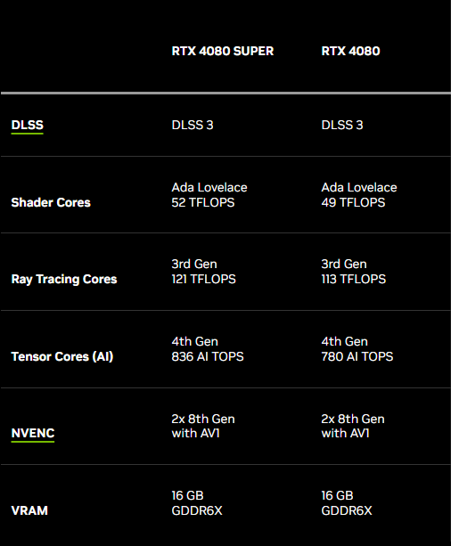
As NVIDIA GPUs are the de facto way to deploy machine learning models as of right now, this post will focus solely on them. We also have to define some specifics about our setup to have any sort of meaningful discussion. In this post, I am specifically talking about CUDA 12.x kernels running on an Ada (ARCH=sm_89) card, because I’m using a RTX 4080 SUPER for the experiments. This architecture can also be found on the RTX 5000 Ada and RTX 6000 Ada cards, among others, and is similar to the Ampere architecture from the famous A100 card.

As a case study, we are going to look at multiplying two $(16384, 16834)$ matrices. This operation might seem arbitrary, but operations like it happen all the time in convolutional layers, linear layers, the attention mechanism, and many others. For instance, it is exactly the last operation that occurs when we calculate self-attention for a sequence of 16384 tokens with a hidden size of 16834. These form the bulk of the computational complexity of using these models.

Just as a warning, I have no delusions of grandeur regarding my abilities in the domain of CUDA programming. Most of my experience lies in designing and training models, not optimizing them. However, I think the latter helps in doing the former two, and optimization is interesting and important in its own right, so I have accrued some familiarity. If you want the raw, unfiltered and all-encompassing details about CUDA programming, the CUDA C Programming Guide is the resource you’re looking for. This post is about what someone with similar experiences to mine might find useful within its 604 pages.

Warmup

As is common knowledge, GPUs are quite good at doing matrix multiplications. After all, they were originally designed for graphics processing, which all boils down to linear algebra. Conveniently (or perhaps consequently), this is also the case for neural networks. A linear layer is just one matrix-matrix multiplication, whereas a convolutional layer is just many smaller matrix-matrix multiplications. Adding a bias, a linear layer is just one matrix-matrix multiplication and one matrix-matrix addition, whereas a convolutional layer is many smaller versions of this. As a blanket statement, one could argue that machine learning models are just matrix multiplications and additions. Despite the statement’s overly simplistic nature, you can get a feel for the part of it that is rather factual by looking at the example model built in my earlier post.

Switching from the mathematical notation to computational terms, this is all just one operation. More specifically, both the multiplication and addition are contained within one GEneral Matrix Multiplication (GEMM): $C = \alpha AB + \beta C$. In matrix multiplication without addition, the scaling parameter $\beta$ is set to zero. In the case of both multiplication and addition, the scaling parameters $\alpha$ and $\beta$ are both set to one. In the case of scaled multiplication and/or addition, the parameters are discretionary.

As an exercise to get into the right mental model, let’s say we have this matrix:

\[\begin{bmatrix} a_{1,1} & a_{1, 2} & a_{1, 3} & a_{1, 4} \\ a_{2,1} & a_{2, 2} & a_{2, 3} & a_{2, 4} \\ a_{3,1} & a_{3, 2} & a_{3, 3} & a_{3, 4} \\ a_{4,1} & a_{4, 2} & a_{4, 3} & a_{4, 4} \\ \end{bmatrix}\]

Matrix multiplications between large matrices can be broken down into many multiplications between small patches of the large matrices. We can turn this $(4, 4)$ matrix into a $(2, 2)$ block matrix, whose elements themselves are $(2, 2)$ matrices:

\[\begin{bmatrix} A & B \\ C & D \\ \end{bmatrix} \text{, such that} \\ A = \begin{bmatrix} a_{1, 1} & a_{1, 2} \\ a_{2, 1} & a_{2, 2} \\ \end{bmatrix} B = \begin{bmatrix} a_{1, 3} & a_{1, 4} \\ a_{2, 3} & a_{2, 4} \\ \end{bmatrix} C = \begin{bmatrix} a_{3, 1} & a_{3, 2} \\ a_{4, 1} & a_{4, 2} \\ \end{bmatrix} D = \begin{bmatrix} a_{3, 3} & a_{3, 4} \\ a_{4, 3} & a_{4, 4} \\ \end{bmatrix}\]

Now, calculating this matrix’s product with itself can be performed as follows:

\[\begin{bmatrix} AA + BC & AB + BD \\ CA + DC & CB + DD \\ \end{bmatrix}\]

The result will be equal to multiplying the original matrix with itself, regardless of its dimensionality. This also applies to multiplying two different matrices, including ones that differ in dimensions. If the dimensions of the multiplied matrices are not divisible by the shape of our submatrices, we can pad them with zeroes while retaining the correctness of our results. For instance, a $(3, 3)$ matrix could be padded as follows to accomodate our $(2, 2)$ submatrices.

\[\begin{bmatrix} a_{1,1} & a_{1, 2} & a_{1, 3} & 0 \\ a_{2,1} & a_{2, 2} & a_{2, 3} & 0 \\ a_{3,1} & a_{3, 2} & a_{3, 3} & 0 \\ 0 & 0 & 0 & 0 \\ \end{bmatrix}\]

However, this doesn’t do much for us on the surface. The number of operations remains constant, we’re just doing them in a different order. In fact, we might end up doing a few extra operations. And this is true, as long as we are calculating the submatrices $A, B, C$ and $D$ sequentially or concurrently. However, things would change if we could calculate them in parallel.

While this isn’t done explicitly during a GEMM in a GPU, these sorts of divide-and-conquer-esque ideas propagate throughout the real process. The way hardware can be built sometimes even means that we end up doing things that are not optimal in mathematical terms, but produce better results in practice [2]. With the orientation behind us, let’s start digging into what CUDA parallelization actually entails.

CUDA bootcamp

Modern NVIDIA GPUs have RayTracing (RT) cores, CUDA cores and tensor cores (since 2017’s Volta architecture). RT cores have no relevance in this discussion, but GEMMs in single-precision (32 bits) or double-precision (64 bits) are generally performed with CUDA cores. CUDA cores perform basic arithmetic, mainly additions, multiplications and their combination called a Fused Multiply-Add (FMA), on scalar data. On the other hand, in modern GPUs, mixed precision GEMMs are best handled by tensor cores. Here, mixed precision could mean 16-bit FP since Volta, 8-bit FP since Ada or 4-bit FP since the Blackwell architecture that is rolling out at the time of writing. Tensor cores are specifically built for performing matrix-matrix multiplications and additions in mixed precision, and therefore work on entire blocks of scalar data at once.

CUDA cores are used for graphics processing and scientific computing, as the full 32-bit precision or even 64-bit precision is often required in these domains. Operations that cannot be formulated in terms of the previously mentioned block matrices are also executed by CUDA cores. For example, the element-wise addition of two FP16 tensors or row-wise matrix-vector addition would be performed by CUDA cores, rather than tensor cores. Language models, along with many others, usually do just fine with 16, 8 or even 4 bit weights. Many are even trained specifically for such precisions. The components within them that carry any sliver of computation complexity can also be formulated as simple GEMMs. Therefore, tensor cores are the ones that get saturated by our machine learning models, and as such we’re going to be focusing solely on them in this post.

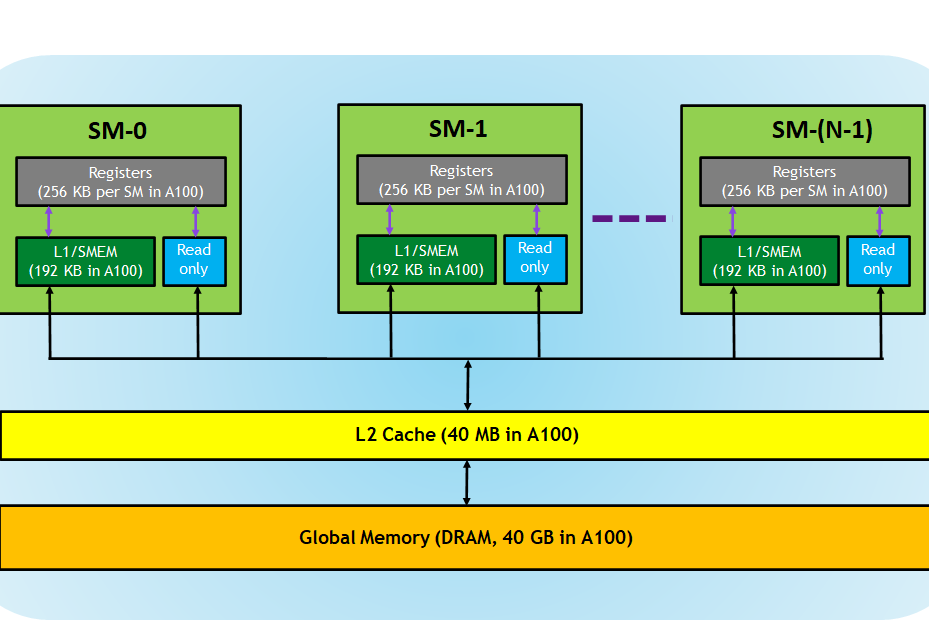
When two matrices $A$ and $B$ are multiplied, the memory for them and the resulting matrix $C$ are allocated in the part of the GPU’s memory that is visible to all processing units, the global memory. This is the VRAM whose size is advertised on all GPUs. Here is a diagram of the full memory hierarchy of a A100 card:

The contents of the matrices $A$ and $B$ which reside on the host (ie. the system RAM) are then loaded into their respective memory locations on the device (ie. the VRAM). If we’re performing matrix-matrix multiplication without addition, the matrix $C$ will be initialized with zeroes directly in VRAM. If we also want to perform addition, we’re going to initialize $C$ with the contents of the matrix we’re using for addition, such that our in-place GEMM $C = \alpha AB + \beta C$ carries out both operations. Here’s some boilerplate that takes care of this process, with the matrix addition omitted. This code will be reused in all subsequent experiments.

#include <cstdio>
#include <cstdlib>
#include <cuda_fp16.h>
#include <cuda_runtime.h>
#include <mma.h>

using namespace nvcuda;

// Input matrix dimensions
#define M_DIM 16384
#define N_DIM 16384
#define K_DIM 16384

int main() {
  size_t bytesA = M_DIM * K_DIM * sizeof(half);
  size_t bytesB = K_DIM * N_DIM * sizeof(half);
  size_t bytesC = M_DIM * N_DIM * sizeof(float);

  // Allocate the required memory on host
  half *h_A = (half *)malloc(bytesA);
  half *h_B = (half *)malloc(bytesB);
  float *h_C = (float *)malloc(bytesC);

  // Initialize A and B to all ones for simplicity
  for (int i = 0; i < M_DIM * K_DIM; i++)
    h_A[i] = __float2half(1.0f);
  for (int i = 0; i < K_DIM * N_DIM; i++)
    h_B[i] = __float2half(1.0f);

  // Allocate the required memory on device
  half *d_A, *d_B;
  float *d_C;
  cudaMalloc((void **)&d_A, bytesA);
  cudaMalloc((void **)&d_B, bytesB);
  cudaMalloc((void **)&d_C, bytesC);

  // Copy contents from host matrices A and B to device
  cudaMemcpy(d_A, h_A, bytesA, cudaMemcpyHostToDevice);
  cudaMemcpy(d_B, h_B, bytesB, cudaMemcpyHostToDevice);

  // ... Grid and block dimensions are defined here

  // ... The matrix multiplication itself is performed here
  wmmaKernel<<<gridDim, blockDim>>>(d_A, d_B, d_C);
  cudaDeviceSynchronize();

  // Copy the computed matrix C back to host
  cudaMemcpy(h_C, d_C, bytesC, cudaMemcpyDeviceToHost);

  // Free the device and host memory
  cudaFree(d_A);
  cudaFree(d_B);
  cudaFree(d_C);
  free(h_A);
  free(h_B);
  free(h_C);

  return 0;
}

What happens inside the wmmaKernel is what is going to define our performance characteristics.

For reference, here is an NVIDIA example kernel. It takes in two matrices $A$ and $B$ of exactly the shape $(16, 16)$, and uses a single mma_sync call (from the mma.h header under the nvcuda::wmma namespace) to multiply them. The result is written into the matrix $C$ of identical dimensions, but with 32-bit precision to avoid overflow.

__global__ void wmmaKernel(const half *A, const half *B, half *C) {
  // Declare the WMMA fragments for A, B, and the accumulator.
  fragment<matrix_a, 16, 16, 16, half, row_major> aFrag;
  fragment<matrix_b, 16, 16, 16, half, col_major> bFrag;
  fragment<accumulator, 16, 16, 16, float> cFrag;

  // Initialize the accumulator fragment to zero.
  fill_fragment(cFrag, 0.0f);

  // Load the 16x16 tile of matrix A.
  load_matrix_sync(aFrag, A, 16);

  // Load the 16x16 tile of matrix B.
  load_matrix_sync(bFrag, B, 16);

  // Perform the matrix multiplication itself using tensor cores.
  mma_sync(cFrag, aFrag, bFrag, cFrag);

  // Store the computed tile back to global memory in row-major order.
  store_matrix_sync(C, cFrag, 16, mem_row_major);
}

This is of course limited and does not make us of all our compute resources, but it doesn’t need to. Afterall, we’re multiplying very small matrices that have a constant size.

Let’s now increase the dimensions of our matrices to the $(16384, 16384)$ mentioned earlier. When using CUDA C++ WMMA and matrices in FP16, the supported dimensions for the inputs of mma_sync are as follows:

$(16, 16, 16)$

$(32, 8, 16)$

$(8, 32, 16)$

We can only perform so much work in one operation. This is by design, of course, as the compiler can’t do all the parallelization for us. Instead, it gives us a toolbox full of useful building blocks, and we can take it from here.

Let’s get one important term out of the way first: Streaming Multiprocessor (SM). SMs are something similar to the idea of cores in CPUs: they have their own registers, caches (shared memory, L1 and a few others), a scheduler to fetch+execute instructions, and many instruction execution pipelines. The CUDA and tensor cores reside within SMs, and are themselves more akin to floating-point units than CPU cores. So don’t think of tensor cores as being similar to CPU cores; the SMs would be a much more fitting comparison out of the two.

Here’s two important diagrams, both from the Ada architecture whitepaper:

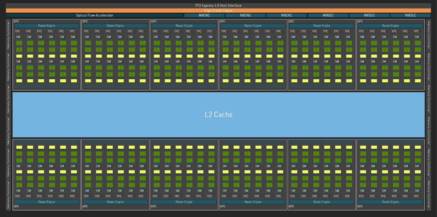
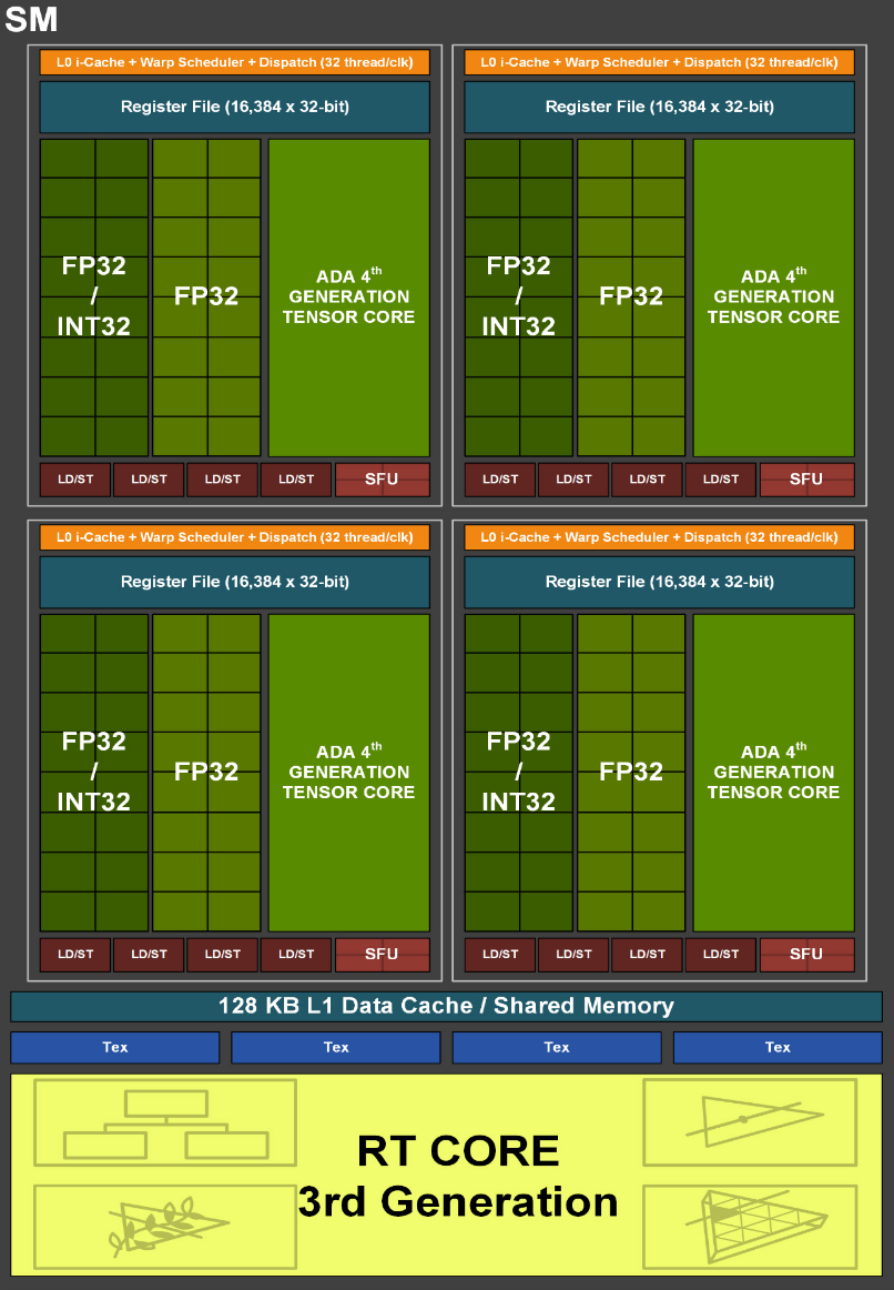
The first is a diagram of the entire architecture. It shows the twelve Graphics Processing Clusters (GPC), that contain six Texture Processing Clusters (TPC) each, that in turn house two SMs each. This is the hierarchy that we are working with. The second diagram zooms into one of these SMs. We can see that each SM contains some FP32/INT32 and FP32 units. These are the CUDA cores, which we will not be using all that much. Then we have the tensor cores, which will do all the heavy lifting in our exercise. Our task is to express our problem in a way that gives all of these SMs with their tensor cores something to do at the same time.

Thinking back to the warmup example, let’s divide the matrix $C$ into smaller parts, which we can then process in parallel. In CUDA terminology, these parts are called tiles, and they are computed with thread blocks, sometimes also known as CUDA blocks. Each of our tiles gets assigned to a single thread block. Each thread block is run dynamically on whichever SM has capacity. Notice that SM is singular; a thread block is run on one and only one SM. All SMs within any given GPU are identical, and can run different thread blocks concurrently but not in parallel. If we launch just one thread block, we’re utilizing just one of our SMs, which is obviously no good. Thread blocks are grouped into a grid, and each thread block contains a set number of warps. A warp is just NVIDIA’s way of saying “a collection of 32 threads executing the same instruction”. We will come back to the definition of threads in just a bit.

So any function (kernel) that we want to run on a GPU is executed on a grid of thread blocks, containing warps, which in turn contain 32 threads. If you are not familiar with CUDA programming, I would recommend reading that sentence a couple of times so these associations become automatic.

Probing for bottlenecks

Obviously, there is going to be some sort of performance limit on a GPU. Here’s a table of some relevant limits on NVIDIA A100:

Max warps / SM	64
Max threads / SM	2048
Max thread blocks / SM	32
Max registers / block	65536
Max registers / thread	255
Max threads / thread block	1024

Unfortunately, I don’t think this sort of a complete table exists for the Ada architecture. The two architectures are not identical either. For instance, each Ada SM can handle at most 24 thread blocks (768 threads) simultaneously, according to the Ada tuning guide. This is in contrast to the 32 threads per Ampere SM.

However, the important idea here is not the specific numbers, but that if one of these inherent limits is reached, our acceleration ends there. We can’t launch more than 768 threads per SM, we can’t perform more than a given amount of clock cycles per second, and so on. Let’s call these the speed limits of the GPU. If one of these speed limits is reached way before the others, we have a bottleneck.

What individual tensor cores actually do

In the Volta architecture, individual tensor cores multiplied two $(4, 4)$ matrices $A$ and $B$, summing their result with another $(4, 4)$ matrix $C$ and then writing it to matrix $D$ in one clock cycle. This is to say, these cores had a $(4, 4, 4)$ processing array that performed an operation called the Matrix-Multiply Accumulate (MMA) on $(4, 4)$ matrices. So in a nutshell, they take two small matrices and perform a multiplication using whatever circuitry NVIDIA has decided to cram into them. They do this in a single clock cycle. The intricate details about the cores are of course not public.

NVIDIA has needed to make their cards faster year-on-year, and there’s really only three ways to do so: increase the clock speed, increase the number of tensor cores and increase the size of this processing array. Here is the progress of these variables going from V100 (Volta) to A100 (Ampere) to H100 (Hopper):

	V100	A100	H100
Boost clock speed	1380 MHz	1410 MHz	1755 MHz
Number of tensor cores	640	432	456
Tensor core processing array size	(4, 4, 4)	(8, 4, 8)	(8, 4, 16)

NVIDIA has so far leaned heavily on increasing the processing array size. After all, if your core can process a matrix twice the size from before each clock cycle, you’ve doubled your throughput. This is even if you keep the other other two variables constant. A doubling of this kind has happened both in the transition from Volta to Ampere and from Ampere to Hopper, with the Ampere architecture doing it in two dimensions simultaneously, resulting in four times the throughput.

It’s important to note that the tensor core processing array size is not something that anyone outside NVIDIA really needs to know, as the CUDA runtime does the mapping from instructions to hardware capabilities. The resulting throughput of these cores is measured in FLoating point Operations Per Second (FLOPS), a common measure for how quickly these cards can do basic math operations. It’s unit is the FLOP, meaning one of these floating point operations, and how many FLOPs a card can do is equivalent to its FLOPS [1]. You really just need to know this number to know how cards stack up against each other, as long as you have an optimized workload. NVIDIA also makes finding these details quite tricky. The specifics were still given out briefly in the A100 whitepaper, but not even mentioned in the Ada whitepaper or the H100 whitepaper. Interestingly enough, the best way to extract these hardware capabilities is to read between the lines when looking at these funky figures put out by NVIDIA:

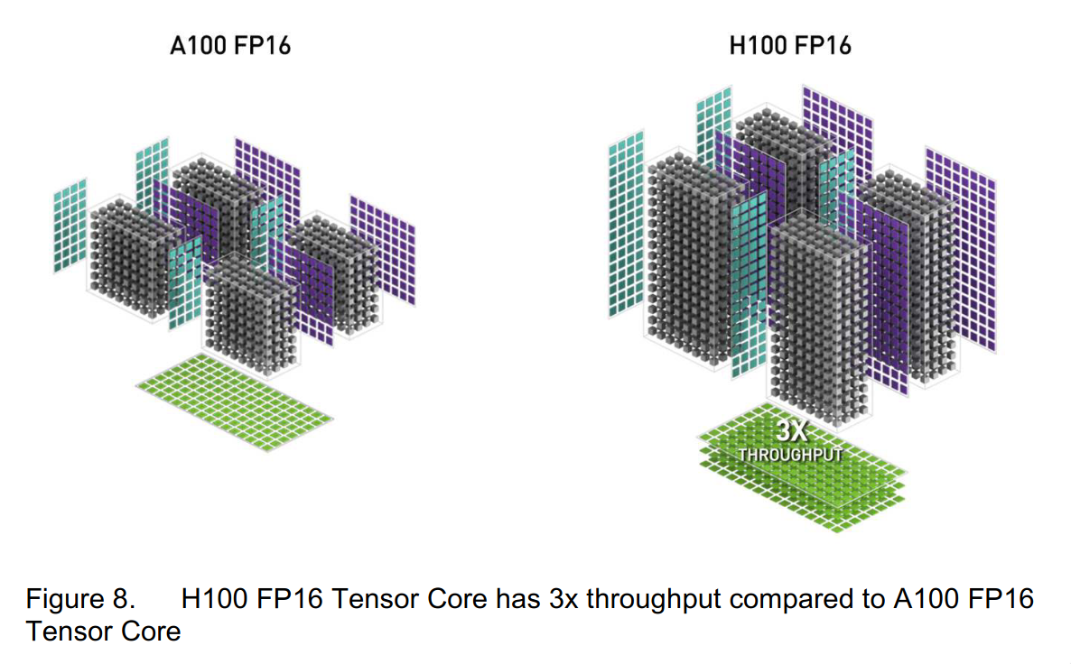
You can see the grey boxes stand for the sizes of the processing arrays, so we are looking at four tensor cores. We can see that the processing arrays have doubled in “height”, so we have gone from $(8, 4, 8)$ to $(8, 4, 16)$. Each tensor core is processing twice the number of datapoints per cycle, so twice the throughput. If you’re wondering why the figure then says 3x and not 2x, the whitepaper confirms the latter figure by stating that the tensor core architecture of the H100 “delivers double the (…) matrix math throughput (…) compared to A100”. However, emboldened by the slightly increased clock speed, the marketing team decided to use 3x in the figure.

In the RTX PRO 6000 card that is currently launching, housing the Blackwell architecture, the number of tensor cores has now doubled to 752, while the boost clock speed has also increased by 50% to 2617 MHz. There is no mention of FP16 performance in the Blackwell whitepaper, with the main focus on how the tensor cores process FP4 data. There’s two possible reads of this situation: this is either a sign of changing strategies, where NVIDIA only increased the clock speed and number of cores, or a sign that NVIDIA is finally throwing the entire kitchen sink at the problem and are just being uncharacteristically quiet about it. If I had to guess, I’d guess the former.

I have no idea how things are going to change in the future, but these types of considerations are definitely something you should look at if you’re in charge of making purchasing decision. However, they’re not really important if you already have the card or cards on hand. As a general rule: just keep the matrix sizes as powers of two and you should be good to go. This way, the small processing arrays of your tensor cores are not filled with redundant zeros. If you’re still not hitting the speed advertised in your card’s spec, consult the tuning guide for your specific GPU.

What’s our hard ceiling?

Now that we have the prerequisite definitions out of the way, let’s briefly return to our discussion on bottlenecks. The number of tensor cores, together with the clock speed and processing array size, define a hard ceiling for how fast meaningful work can be performed. The RTX 4080 SUPER is operating at a (base) clock speed of 2295 MHz, so around 2 billion clock cycles a second. It also has 80 SMs with 4 tensor cores each, meaning a total of 320 tensor cores. So each of our tensor cores could theoretically be performing MMAs 2 billion times per second, and this multiplied with 320 would be our throughput.

As mentioned before, the Ada whitepaper makes no mention of the processing array’s size. The entire section on the tensor cores is less than 100 words long. However, it does mention that: “Compared to Ampere, Ada delivers more than double the FP16 (…) Tensor TFLOPS”. We know that NVIDIA’s more than double just means exactly twice as much, so we can assume that the processing array has doubled in size. This doubling was marketed as being new in the Hopper lineup, but this is just because all the benchmarks compared the new cards against an A100, and not the actual previous generation (ie. Ada). You can see this in action in the Figure 8 from above.

But now we know that our processing array size is in fact $(8, 4, 16)$. Therefore, as each MMA contains 16 FMAs per value in the resulting $(4, 8)$ matrix, and each FMA performs two FLOPs (multiplication and addition), each MMA computes 1024 FLOPs. Therefore, our theoretical limit would be $2295 \cdot 10^6 \cdot 320 \cdot 1024 = 8.35584 \cdot 10^{14}$ FLOPS, or rougly $836$ TFLOPS. As we are using tensor cores, NVIDIA would refer to these numbers as Tensor Operations Per Second (TOPS) or AI TOPS. Whenever you come across this marketing buzzword, just know that it’s the exact same thing as TFLOPS. We can see that the numbers we got are the same ones touted by NVIDIA, at around 836 AI TOPS:

The reason I refer to this as a hard ceiling is that even if this sort of throughput would theoretically be possible with the given tensor cores, it’s not at all realistic. This is due to overhead from scheduling, data transfer and so on, especially as the multiplied matrices grow in size. To emphasize just how theoretical this limit is: 836 TFLOPS would be equivalent to calculating the matrix multiplication of two $(\sqrt[3]{\frac{835.584 \cdot 10^{12}}{2}}, \sqrt[3]{\frac{835.584 \cdot 10^{12}}{2}}) = (74757, 74757)$ matrices every second. The resulting matrix would have around 5 600 000 000 values. As you’ll see, we won’t get even close to this in the real world.

Performing the calculations

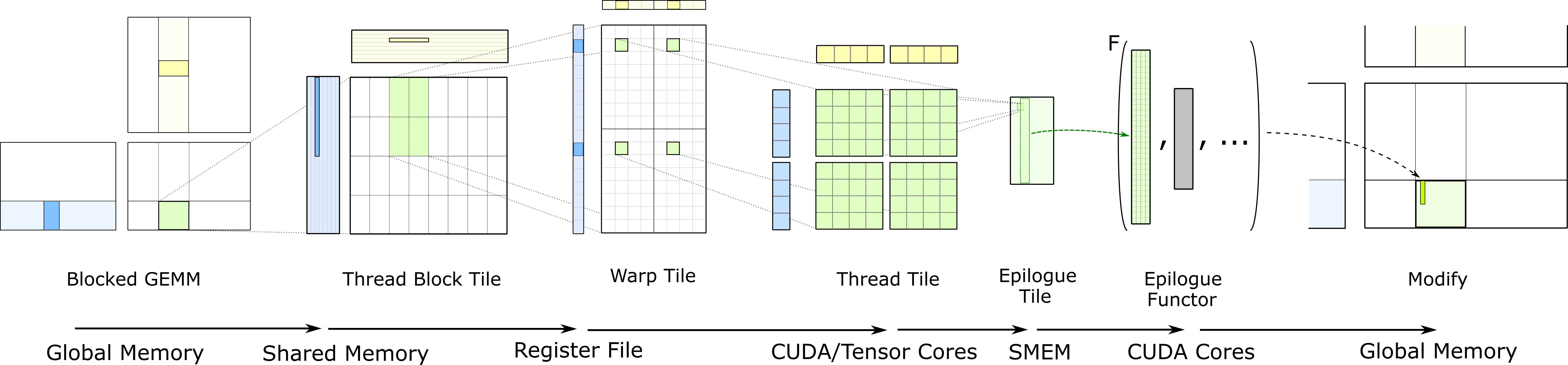
Let’s now dig into how these GEMMs should be formulated, such that we make our SMs busy. Here’s a visual aide:

On a high level, the green rectangle is one of our tiles. Stepping through the K dimension, we take $\mathbb{R}^{M \times K}$ and $\mathbb{R}^{K \times N}$ sized chunks from the matrices $A$ and $B$ respectively, and multiply them. The result is summed directly into the matrix $C$, usually in 32 bit precision to avoid overflow.

In the following discussion, let’s assume the $(4, 4, 4)$ processing array from the Volta architecture, as its squareness lets us keep the discussion a bit more focused. Going through this process in more detail:

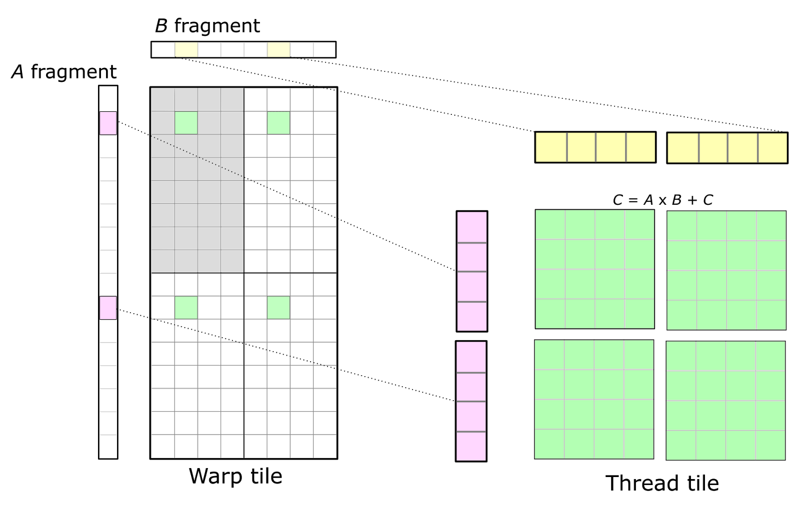
Each tensor core calculates 16 values per clock cycle, each of which is the result of four FMA operations (as they are the results of dot products between the rows and columns with 4 elements each). A single warp produces an accumulator tile of some dimensions. This is to say, a (small) patch of the matrix $C$. A single warp would be a quadrant in the warp tile visualization of the above image. The cells are the threads, of which we know there to be 32. The reason for having a unit such as a warp is that it allows us to schedule work in atomic pieces. We start 32 threads at once, each of which runs the exact same instructions on its respective data. The image above zooms into four of these warps, but all of them should be running in lock-step. This way we can get the most mileage out of the rows from $A$ and columns from $B$ that we have now loaded in the L2 cache.

As is evident, computation can be split into three levels: parallelization between thread blocks, warps and individual tensor cores. Zooming into the visualization after the warp tile, we have a tile of what is essentially the smallest unit of work that runs a piece of kernel code: threads.

Each thread has its own registers and a tiny bit of memory that is local to itself. So when you write a kernel, it gets compiled into instructions; A thread is the unit that executes one of these instructions at a time. Obviously, if a row from A is required by 10 of these warps, we’d like for that row to be loaded into the L2 cache only once, and for all 10 warps to perform their work in parallel when that happens. But the important bit here is that these thread blocks, with their warps and ultimately threads, are not actually dependent on each other; they can all be run at the same time. This is why we are able to make use of this massive pool of tensor cores.

In this sea of complexity, one important detail is that the kernel code does not need to (and in fact cannot) define which hardware units execute any given instruction. This is the job of the compiler, the CUDA runtime and the hardware itself. By compiling a program that includes a kernel using mma_sync on two matrices of correct dimensions and data type, the compiler writes instructions that make the CUDA runtime spawn thread blocks, which the card’s global scheduler then allocates to SMs. The warp schedulers inside the SMs then decide which warps are being run and when, possibly switching between them on the fly. The SMs have a hardwired pipeline for all instructions executed by the warp, and when the instructions related to our mma_sync come up they are then directed to the tensor cores. At no point does the CUDA developer need to specify hardware units or instruction pipelines, but being aware of them is fundamental to writing performant CUDA kernels.

Getting our hands dirty

Let’s actually look at what this kind of kernel code looks like. Here’s the basic design for our first kernel:

• The multiplied matrices are $A, B \in \mathbb{R}^{16384 \times 16384}$, represented by floating point values in 16-bit precision.
• The result matrix is $C \in \mathbb{R}^{16384 \times 16384}$, represented by floating point values in 32-bit precision.
• The calculation is split into thread blocks, each consisting of one warp (32 threads).
• Each thread block computes a $(16, 16)$ tile of $C$.
  • Therefore, the grid is ($\frac{16384}{16}$, $\frac{16384}{16}$) = (1024, 1024).
• Each warp calculates one $(16, 16)$ tile of $C$.
• In total, 1 048 576 thread blocks, 1 048 576 warps and 33 554 432 threads. The matrix $C$ has a total of 268 435 456 elements.

And here is the code for it:

// ... Same as before

// Each WMMA operation works on a 16x16 tile with a K-dimension of 16.
#define WMMA_M 16
#define WMMA_N 16
#define WMMA_K 16

__global__ void wmmaKernel(const half *A, const half *B, float *C) {
  const int lda = K_DIM; // row-major
  const int ldb = K_DIM; // column-major
  const int ldc = N_DIM; // row-major

  // The grid is organized in warp tiles, where each warp covers one 16x16 tile
  int warpM = blockIdx.y;
  int warpN = blockIdx.x;

  // Declare fragments for a 16x16 tile
  wmma::fragment<wmma::matrix_a, WMMA_M, WMMA_N, WMMA_K, half, wmma::row_major>
      aFrag;
  wmma::fragment<wmma::matrix_b, WMMA_M, WMMA_N, WMMA_K, half, wmma::col_major>
      bFrag;
  wmma::fragment<wmma::accumulator, WMMA_M, WMMA_N, WMMA_K, float> accFrag;

  // Initialize the output to zero
  wmma::fill_fragment(accFrag, 0.0f);

  // Loop over the K dimension, biting off a WMMA_K sized chunk each time
  for (int k = 0; k < K_DIM / WMMA_K; ++k) {
    // This gets a bit confusing so let's clarify with comments...

    // A is row-major, so:
    // * A[i][j] is stored at A[i * lda + j]
    // * Starting "row" index (i) is warpM * WMMA_M
    // * Starting "column" index (j) is k * WMMA_K
    const half *tileA = A + warpM * WMMA_M * lda + k * WMMA_K;

    // B is column-major, so everything is flipped:
    // * B[i][j] is stored at B[i + j * ldb]
    // * Starting "row" index (i) is k * WMMA_K
    // * Starting "column" index (j) is warpN * WMMA_N
    const half *tileB = B + k * WMMA_K + warpN * WMMA_N * ldb;

    // Load the tiles into WMMA fragments.
    wmma::load_matrix_sync(aFrag, tileA, lda);
    wmma::load_matrix_sync(bFrag, tileB, ldb);

    // Perform the MMA using tensor cores.
    wmma::mma_sync(accFrag, aFrag, bFrag, accFrag);
  }

  // Store the computed 16x16 tile back to C.
  float *tileC = C + warpM * WMMA_M * ldc + warpN * WMMA_N;
  wmma::store_matrix_sync(tileC, accFrag, ldc, wmma::mem_row_major);
}

int main() {
  // ... Same as before

  // Set up grid and block dimensions
  // Grid:
  //    One block per 16x16 tile of C ==> (16384/16) x (16384/16) = (1024, 1024)
  // Block:
  //    One warp per block -> 32 threads
  dim3 gridDim(N_DIM / WMMA_N, M_DIM / WMMA_M);
  dim3 blockDim(32, 1, 1);

  // ... Same as before
}

For the sake of benchmarking, let’s wrap the wmmaKernel call into a loop of 10 iterations:

// PC case turbine activator
for (int i = 0; i < 10; ++i) {
  wmmaKernel<<<gridDim, blockDim>>>(d_A, d_B, d_C);
  cudaDeviceSynchronize();
}

Now, let’s compile and run it with nvcc -arch=sm_89 wmma_gemm.cu -o ./wmma_gemm && time ./wmma_gemm. The runtime is about 33.1 seconds. Not bad for calculating around 270 million elements worth of matrix multiplication.

This is quite alright for a first attempt, but we’ve made a questionable decision: There’s only one warp per thread block, and each thread block calculates only a $(16, 16)$ tile of $C$. This has led to an explosion in the number of warps, and therefore threads, and the SM can’t switch between warps to hide latency. The scheduling of this is also bound to cause some overhead, and we’re definitely hitting one of the previously mentioned speed limits. Let’s see if we can do a better by launching, say, 4 warps per thread block and increasing the thread block tile size appropriately:

• The multiplied matrices are (still) $A, B \in \mathbb{R}^{16384 \times 16384}$, represented by floating point values in 16-bit precision.
• The result matrix is (still) $C \in \mathbb{R}^{16384 \times 16384}$, represented by floating point values in 32-bit precision.
• The calculation is split into thread blocks, each consisting of four warps (128 threads).
• Each thread block computes one $(64, 64)$ tile of $C$.
  • Therefore, the grid is ($\frac{16384}{64}$, $\frac{16384}{64}$) = (256, 256).
• Each warp calculates four $(16, 16)$ tiles of $C$.
• In total, 65 536 thread blocks, 262 144 warps and 8 388 608 threads. The matrix $C$ (still) has a total of 268 435 456 elements.

Here’s the updated kernel:

// ... Same as before

// We split the result matrix into 64x64 tiles per thread block.
#define BLOCK_TILE_M 64
#define BLOCK_TILE_N 64

// The grid is 256x256
// Each block computes a 64x64 region of C, spanning the entire 16384x16384
// matrix. Within a block, its 64x64 tile is made of 4x4 WMMA sub-tiles, each
// of size 16x16. There are 4 warps (128 threads) per block. Each warp handles
// one "row" of the WMMA sub-tiles.
__global__ void wmmaKernel(const half *A, const half *B, float *C) {
  const int lda = K_DIM; // row-major
  const int ldb = K_DIM; // column-major
  const int ldc = N_DIM; // row-major

  // The starting coordinates of this block's tile in matrix C
  int block_row = blockIdx.y * BLOCK_TILE_M;
  int block_col = blockIdx.x * BLOCK_TILE_N;

  // Within the block, launch 4 warps -> 128 threads.
  // Each warp computes a 16-row & 64-column strip of the full 64x64 tile, in
  // four batches of 16x16 sub-tiles
  int warpId = threadIdx.x / 32; // 0 .. 7

  // Global row offset for what is computed by this warp
  int global_row = block_row + warpId * WMMA_M;

  // Each warp computes 4 WMMA tiles along the column direction, so we need
  // an array of accumulator fragments: one for each of the 4 sub-tiles in this
  // warp's row.
  wmma::fragment<wmma::accumulator, WMMA_M, WMMA_N, WMMA_K, float> acc_frag[4];

  // Barrel roll
  #pragma unroll
  for (int i = 0; i < 4; i++) {
    wmma::fill_fragment(acc_frag[i], 0.0f);
  }

  // Loop over the K dimension, biting off a WMMA_K sized chunk each time
  for (int k_tile = 0; k_tile < K_DIM / WMMA_K; k_tile++) {

    // Each warp first loads its fragment in A
    wmma::fragment<wmma::matrix_a, WMMA_M, WMMA_N, WMMA_K, half,
                   wmma::row_major>
        a_frag;

    // A is row-major, so:
    // * A[i][j] is stored at A[i * lda + j]
    // * Starting "row" index (i) is the global row computed above
    // * Starting "column" index (j) is k_tile * WMMA_K
    const half *tileA = A + global_row * lda + k_tile * WMMA_K;

    wmma::load_matrix_sync(a_frag, tileA, lda);

    // Now, loop over the 4 sub-tiles in columns that this warp is responsible for
    #pragma unroll
    for (int i = 0; i < 4; i++) {
      // Global column offset for this WMMA tile
      int global_col = block_col + i * WMMA_N;

      // Load the fragment from B
      wmma::fragment<wmma::matrix_b, WMMA_M, WMMA_N, WMMA_K, half,
                     wmma::col_major>
          b_frag;

      // B is column-major, so everything is flipped:
      // * B[i][j] is stored at B[i + j * ldb]
      // * Starting "row" index is k_tile * WMMA_K
      // * Starting "column" index is the global column computed above
      const half *tileB = B + k_tile * WMMA_K + global_col * ldb;

      wmma::load_matrix_sync(b_frag, tileB, ldb);

      // Perform the MMA
      wmma::mma_sync(acc_frag[i], a_frag, b_frag, acc_frag[i]);
    }
  }

  // Because the accumulation is done over K, each warp stores its 4 resulting
  // 16x16 tiles
  #pragma unroll
  for (int i = 0; i < 4; i++) {
    // The starting pointer in matrix C for this 16x16 sub-tile
    int global_col = block_col + i * WMMA_N;
    float *tileC = C + global_row * ldc + global_col;

    wmma::store_matrix_sync(tileC, acc_frag[i], ldc, wmma::mem_row_major);
  }
}

int main() {
  // ... Same as before

  // Set up grid and block dimensions
  // Grid:
  //    One block per 64x64 tile of C ==> (16384/64) x (16384/64) = (256,
  //    256)
  // Block:
  //    Four warps per block -> 128 threads
  dim3 gridDim(N_DIM / BLOCK_TILE_N, M_DIM / BLOCK_TILE_M);
  dim3 blockDim(128, 1, 1);

  // ... Same as before
}

Again, let’s wrap this kernel a loop of 10 iterations. Compiling and running with nvcc -arch=sm_89 multiwarp_wmma_gemm.cu -o ./multiwarp_wmma_gemm && time ./multiwarp_wmma_gemm, this takes about 8.7 seconds. Much better.

If we want to, we can fiddle with the number of thread blocks and warps some more. For instance, if we make the following changes:

• Thread block tile size $(64, 64)$ -> $(128, 128)$
• Number of warps per thread block 4 -> 8
  • Number of threads 128 -> 256
• In total, 16 384 thread blocks, 131 072 warps and 4 194 304 threads.

The runtime drops to 6.8 seconds. This is about 13 TFLOPS. Not bad.

And remember, we are calculating the same matrix here. There’s no tradeoffs or shortcuts being taken, the kernel is doing the same computations but with better resource utilization. Also, note that all of these methods use the exact same amount of VRAM and get the GPU to 100% utilization according to tools like nvidia-smi or nvtop (which critically do not measure any sort of core or memory bus saturation).

Simple enough?

Obviously, this explanation hides a mountain of further optimizations, most of which I have no idea about. I can reconsile in the fact that neither does anyone else, as cuBLAS along with its GEMM kernels are not open source.

However, if you are feeling especially curious, the GEMM kernels of CUTLASS are in fact publicly available. A good starting point would probably be its FP8 Ping-Pong kernel, whose way of combining three warps blows many others out of the water in terms of tensor core utilization:

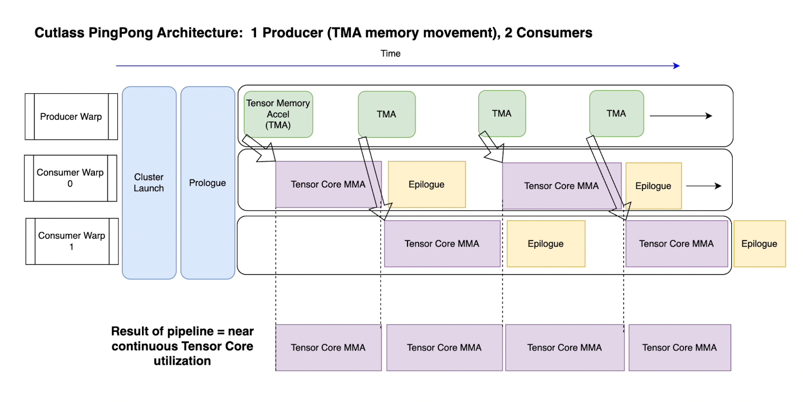
To give an example of some of the things that are out there: double buffering is a technique used to perform computations on one buffer of data while another buffer is being loaded. So instead of load-compute-unload, all three steps are running in an intertwined fashion. This blurs the line between data transfer and computation, reducing the number of cycles where the cores just idle while waiting for new data to arrive. You won’t get anything close to the promised performance on a GPU without something like this.

Real world woes

It is worth pointing out that many machine learning models are not actually compute-bound. This is to say, the GPU is not carrying out as many MMA computations as it could at any given time. Instead, the speed at which data can be transferred from VRAM to caches forms a bottleneck. This is a diagram from the Activation-aware Weight Quantization (AWQ) paper:

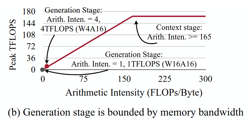
As the authors put it:

The 4090 GPU has a peak computation throughput of 165 TFLOPS and a memory bandwidth of 1TB/s. Therefore, any workload with arithmetic intensity (the ratio of FLOPs to memory access) less than 165 is memory bounded on 4090 GPUs.

If the number of FLOPs performed using any given byte of information multiplied by the memory bandwidth is not higher than the card’s FLOPS rating, we will always be leaving performance on the table. This is solely by virtue of the data not getting to the computational units fast enough for them to actually have to sweat. Whenever we bring a byte through the memory bus, we never do enough things with it for the cores to get saturated. There’s really just three fixes: increase the memory speed, increase the number of FLOPs per byte or reduce the number of bytes per FLOP. At the moment, NVIDIA is advocating for the first with their ever speedier DRAM and the last with their new FP4 tensor cores.

There’s also an extreme version on this, where the GPU is not spending most of the time even performing MMAs. Clearly, the data transfer is never going to be instant, and therefore the cores are not going to be at full saturation at all times, but this is different: the GPU is mostly just accessing memory. NVIDIA calls this being memory limited, instead of math limited.

The generation stage of large language models is generally memory-bound. The reason is that you are generating just one token at a time, ie. using batch size of one. Remember that the KV cache retains the inter-layer representations of the prior tokens, so they are are not calculated again. This simply does not entail enough raw computations to saturate the cores, given how much data you have to move around. In an encoder-only language model, on the other hand, the arithmetic intensity is on par with the context stage of large language models. This is because we are processing the entire token sequence at the same time, instead of one token at a time. In attention layers, we are calculating the attention values between all of our tokens, not just the attention values between the last token and all the previous ones.

Just so I can provide at least some solutions and not just problems: if you have multiple generations ongoing at the same time, you can process the next-token prediction for all of them as one batch. This is one of the reasons online chatbots sometimes wait before beginning to answer even the shortest of questions. The server is waiting for requests from other people to fill a batch, so that they don’t underutilize their GPUs.

There are also application specific optimizations, such as FlashAttention and FlashAttention-2 for how the matrix multiplications within an attention block should be performed. These are not optimizing how one GEMM should be performed, but how multiple GEMMs (mixed with other transforms such as softmax) should be performed together. Such kernels are known as fused kernels, kernels that perform the job of multiple kernels at once. The optimizations of FlashAttention mostly come from memory access patterns that lead to better utilization of the on-chip memory (SRAM) instead of the DRAM. This means that while transferring a byte of information through the memory bus takes the same amount of time, we are performing more useful work on said byte once it has made this trip. Instead of repeatedly reading that byte from DRAM, it stays in SRAM. This was the third way to improve memory-bound inference. For a more in-depth look at how the fused kernel in FlashAttention-2 works, AMD’s ROCm blog has a great article on implementing it.

So, if you’re investigating performance of autoregressive models or models that have an otherwise low arithmetic complexity, you might want to consider these things before attempting to optimize the math.

Is our kernel actually any good?

For the sake of comparison, let’s try some alternatives to our kernel that are also a bit easier to reason about. CUTLASS provides a python library that should be using all of their highly optimized kernels. Let’s see how this goes:

from time import sleep, time

import cutlass
import numpy as np

size = 16384
plan = cutlass.op.Gemm(element=np.float16, layout=cutlass.LayoutType.RowMajor)
A, B = [np.ones((size, size), dtype=np.float16) for _ in range(2)]
C, D = [np.zeros((size, size), dtype=np.float32) for _ in range(2)]

for _ in range(10):
    plan.run(A, B, C, D)

The runtime is 16.75 seconds. Ouch. Even when timing just the calls to plan.run(), sidestepping potential GIL lock slowdowns and memory allocations at the start, the runtime is about 11.8 seconds. However, this approach does seem to deallocate & allocate the ~3 GiB of VRAM used by the GEMM between each of the loop’s iterations. That’s definitely affecting the results. I’m sure there’s a better way to do this using CUTLASS, but let’s check out how well torch does out of the box with a similar piece of code:

import torch

size = 16384
A, B = [torch.ones([size, size], dtype=torch.float16, device="cuda") for _ in range(2)]

for i in range(10):
    C = A @ B

1.9 seconds.

Even when initializing the matrices $A$ and $B$ to random floating point values, the runtime stays the same. So there aren’t any tricks here that rely on the values of the matrix being zero - it actually is that fast. Let’s find out just how fast exactly.

from time import time
import torch

size = 16384

start = time()
for i in range(350):
    A, B = [
        torch.randn([size, size], dtype=torch.float16, device="cuda") for _ in range(2)
    ]
    C = A @ B
end = time()
print(end - start)

We’re re-initializing the values of the matrices during each iteration of the loop from a standard normal distribution (within the python interpreter), and running the loop 350 times.

The runtime of this is rougly 8 seconds. As such, we are reaching about $\frac{16384^3 \cdot 2 \cdot 350}{8} = 3.85 \cdot 10^{14}$ FLOPS, ie. 385 TFLOPS. The GPU pulls an enormous 319W from the PSU and kicks the fans to high speed. The maximum rated wattage of the card is 320W. This is not even half of our rated 836 AI TOPS, but it’s probably close to the card’s realistic limit. How is this possible? Well, internally torch uses the kernels from cuBLAS. It is truly crazy how fast those things are, even when burdened by being run from inside an interpreted language. For comparison, my kernel with its 6.8 second runtime for just 10/350 of these GEMMs draws about 175W.

Out of curiosity, I pulled up the first listing from Amazon with the search “electric stove”, which was some sort of a portable device that could bring a single pot to a boil. It had a rating of 500W, not too far off from what the RTX 4080 SUPER consumer while running this simple script.

Closing thoughts

Modern GPUs are able to calculate large matrix-matrix products extremely efficiently, achieving exceptional levels of parallelism. This also applies to other hardware designed for such purposes, such as TPUs or even most CPUs, due to the increasing support for the later AVX extensions to the x86 instruction set, namely AVX-512.

If you’re someone who deals with ML model deployments, you need to be able to make educated guesses about the sort of performance you should be getting. If this expectation is not being met, you then investigate and usually find a mistake on your own part. Life is an exercise in humility, just fix it and move on. If you’re doing something truly novel and the solutions other people have come up with don’t work for you, you can then optimize according to your own judgement. Just don’t fall victim to the hubris of expecting to beat NVIDIA engineers at writing kernels for common operations on their own hardware.

The most important thing to keep in mind is that investigating why memory bandwidth is not being utilized or cores are not saturated is not some sort of magic. Some basic understanding of what the GPU is actually doing goes a long way.

Notes:

The code for these experiments can be found in this Github repository.

[1] Yes, the acronym for FLOPs does not match the actual words it represents, and it simply evolved to mean “the thing whose frequency is measured in FLOPS”, hence the pseudo-backronym. I know it doesn’t make sense, but (unfortunately) that decision was not for me to make.

[2] There is an alternative algorithm to the one you, I or a GPU would use to perform matrix-matrix multiplication. This is known as the Strassen algorithm, and it can reduce the required number of scalar multiplications drastically for large matrices; The number of operations drops from the $O(n^3)$ of triply nested loops down to $O(n^{2.8074})$. The Strassen algorithm has been improved further even as late as 2023, but these improvements have been limited to reducing the number of scalar addition required. The number of scalar multiplications has been known to be optimal since the first improvement to Strassen’s work by Shmuel Winograd. These methods are effectively never used in modern hardware, as the triply nested loop can be implemented and parallelized more effectively in practice.