Birdbrain batching and tips on never using it

\[\require{amsmath}\]

This post is a follow-up to Batching arises naturally from the fundamental design of neural networks. If you’re unfamiliar with neural networks or the concept of batching, I would recommend reading that post first.

When you’re dealing with a traditional neural network, you will have statically sized feature vectors and parallelism will be straightforward. This post is about batching when the inputs to the model are different lengths. One pertinent scenario where this typically occurs is natural language. We will be using a language model consisting of a decoder-only transformer as an example. Here, the differing lengths of the tokenized inputs make batching non-trivial. Numerous other models face this exact same challenge in their respective modality, and I think this challenge can generally be solved in a way that is either clever, industrious or birdbrained.

Let’s go step by step in trying to adapt the straightforward method of traditional neural networks into a transformer that is analyzing the sentiments of movie reviews.

Getting our token sequences

Let’s start with a quick detour into probability theory. We will use this information in order to get some realistic data for our experiments.

A countless number of randomly occurring things in this world produce the exponential distribution. More specifically, any homogeneous Poisson process creates inter-arrival times that form the exponential distribution. Breaking that statement down, a homogeneous Poisson process is simply a random process where in a given interval of time, the probability of an event occurring is proportional to the length of the interval and independent of other intervals. This is a continuous time version of the (discrete) Bernoulli process, where each individual experiment has a (constant) probability of success that is independent of all previous and later experiments; think of a coin flip.

In the Bernoulli, we have discrete events that have a success rate. In the Poisson, we have continuous time intervals that have an arrival rate. A Bernoulli process generates a geometric distribution, whereas a Poisson process generates an exponential distribution.

As an everyday example, let’s say you sit by a highway and spot red cars as they pass by. The probability of seeing at least one red car in a time interval of 5 minutes is, say, 30%. This probability, for any given interval, does not vary based previous or subsequent intervals. Similarly, let’s say that the probability of any given car being red is 5%. This probability, for a given car, does not vary based on the cars around it. The (discrete) number of non-red cars between each spotting of a red car would produce a geometric distribution; The (continuous) lengths of time intervals between red cars would produce an exponential distribution.

You can probably come up with a dozen ways this could be used off the top of your head: customer service request durations, equipment usage times between malfunctions, radioactive decay… If we parameterize the distribution to match our historical data, we can evaluate likelihoods for future events with some degree of confidence. Here, we can use an exponential distribution to model the lengths of our movie reviews. You could just as well (and perhaps more sensibly) use a geometric distribution. In any case, we sample 1000 values from an exponential distribution and discretize them to signify movie review lengths:

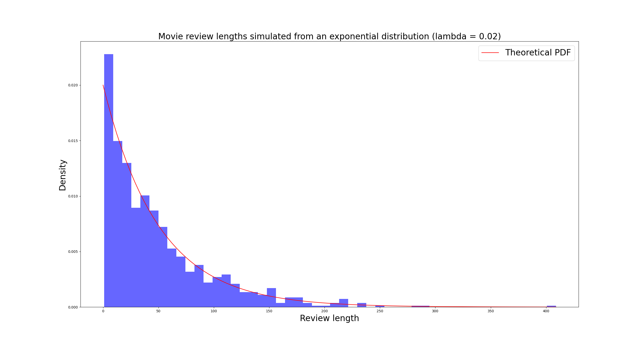
For practical purposes, I’ve turned all the zeroes we sampled into ones. The longest review we got was just about 400 words long, while most of them landed within 1-10 words. The rest of the lengths are scattered around 10-200 in decreasing fashion, with a few popping up between 200 and 400 as well. Makes sense, most people write short reviews, some put in more effort. A handful decide to write a novel.

We will be generating the words of each review randomly up to its respective length.

Optimal brain damage

Let’s say we now have a sentiment analysis model and want to analyze these reviews. Let’s further define that our model’s weights are in half-precision (16 bits). The model consists of the following things:

• Embedding matrix for mapping tokens into embedding vectors
• Multiple blocks made up of a non-masked single-head self-attention layer and a linear layer
• A decision head (just another linear layer), which then maps its input into a vector of two values.
  • The first of these is interpreted as being a measure of positivity, the second as being a measure of negativity. The larger of the two is chosen as our label.

Here is an implementation without any libraries or frameworks (other than for basic linear algebra operations and data types):

hidden_dim = 4096
vocab_size = 65535
num_layers = 70
dtype = float16

class WhateverModel:
    def __init__(self):
        self.padding_token_id = -100

        # Embeddings
        self.embeddings = torch.rand(
            [vocab_size, 1, hidden_dim], dtype=dtype, device="cuda"
        )

        # Attention weights
        self.q_proj_weights = [
            torch.rand([hidden_dim, hidden_dim], dtype=dtype, device="cuda")
            for _ in range(num_layers)
        ]
        self.k_proj_weights = [
            torch.rand([hidden_dim, hidden_dim], dtype=dtype, device="cuda")
            for _ in range(num_layers)
        ]
        self.v_proj_weights = [
            torch.rand([hidden_dim, hidden_dim], dtype=dtype, device="cuda")
            for _ in range(num_layers)
        ]
        self.o_proj_weights = [
            torch.rand([hidden_dim, hidden_dim], dtype=dtype, device="cuda")
            for _ in range(num_layers)
        ]

        # Linear layers
        self.linear_weights = [
            torch.rand([hidden_dim, hidden_dim], dtype=dtype, device="cuda")
            for _ in range(num_layers)
        ]
        self.linear_biases = [
            torch.rand([1, hidden_dim], dtype=dtype, device="cuda")
            for _ in range(num_layers)
        ]

        # Decision head
        self.decision_head = torch.rand([hidden_dim, 2], dtype=dtype, device="cuda")

The model is missing all of the bells and whistles of modern large language models. No grouped query attention, no GeLU (or any other nonlinearity), no residual connections.

This is by design, as we are not trying to build an intelligent model, but a model that embodies the computational burdens of an intelligent model without all the distractions. We have added one component where the tokens are interconnected (self-attention) and one where they are not (linear layer), and that’s it. Consequently, our forward pass is effectively just 7 matrix multiplications, performed for each of our blocks. Goes to show how simple this stuff gets when you remove the cruft.

Here’s the forward pass:

    @staticmethod
    def normalize(X: Tensor):
        mean = X.mean(dim=-1, keepdim=True)
        std = X.std(dim=-1, keepdim=True)
        return (X - mean) / (std + 1e-5)

    def forward(self, documents: list[list[int]]) -> list[bool]:
        X, attention_mask = self.embed_documents(documents)

        attention_mask = attention_mask.unsqueeze(2)
        attention_mask = torch.cat(
            [attention_mask] * attention_mask.shape[1], dim=2
        ).transpose(1, 2)

        for i in range(num_layers):
            # Attention layer
            q_states = X @ self.q_proj_weights[i]
            k_states = X @ self.k_proj_weights[i]
            v_states = X @ self.v_proj_weights[i]

            attn_weights = q_states @ k_states.transpose(1, 2) / math.sqrt(hidden_dim)
            attn_weights += attention_mask
            attn_weights = F.softmax(attn_weights, dim=-1)
            attn_weights = attn_weights @ v_states

            X = attn_weights @ self.o_proj_weights[i]

            # Linear layer
            X = X @ self.linear_weights[i] + self.linear_biases[i]

            # Normalization so the values don't explode
            X = self.normalize(X)

        # Just take the first token's output as a pseudo "class token"
        cls_tokens = (X @ self.decision_head)[:, 0, :]
        decisions: list[bool] = [(tok[1] >= tok[0]).item() for tok in cls_tokens]  # type: ignore

        return decisions

In terms of vocabulary, let’s define that our tokenizer does not map subwords, but only knows whole words. This is just so we don’t have to get bogged down by the token/word distinction.

How a single review gets analyzed

When we have a review that is made up of $100$ words, these words are first mapped into $100$ tokens indices based on our vocabulary. Then, each of these tokens is given an embedding vector simply by looking it up from the embedding matrix. Notice that our model uses an embedding dimension (or hidden dimension) of $4096$. As such, the input to the rest of the model is now of size $\mathbb{R}^{100 \times 4096}$. If you’re unsure about how this matrix makes it through the model, it will be explained in the following paragraph. If you don’t need convincing, feel free to skip it.

The self-attention starts off with three linear layers. These linear layers each multiply our matrix with another matrix whose shape is $\mathbb{R}^{4096 \times 4096}$. No problems there - we will receive a new $\mathbb{R}^{100 \times 4096}$ matrix as a result, keeping the dimensionality unchanged. We now have three new matrices of identical dimensions to the original one. Next, the first of these is multiplied with the second’s transpose, and the result is then multiplied with the third. To quickly convince ourselves that this is fine, we can think of it this way: These three matrices are of the same dimensions and we don’t care about their contents right now, so let’s call them all $\boldsymbol{X}$. It is trivially provable that for any matrix $\boldsymbol{X}$ of arbitrary dimensions, $\boldsymbol{X X^T X}$ will always produce a matrix of identical dimensions to $\boldsymbol{X}$. Therefore, we are once again left with a matrix whose dimensionality is identical to our starting matrix. Then, there is a linear layer whose weight matrix is identically sized to our those of our first three linear layers. We now know that these do not modify the dimensionality of our matrix, so we exit the block with an output whose size is identical to the input. The operations run within the different blocks are identical and the blocks themselves are directly connected to one another, so the matrix passes through all blocks without problems, producing a matrix of identical dimensions every time. The final linear layer has the same amount of rows as the prior ones but only two columns, so it will output a matrix of size $\mathbb{R}^{100 \times 2}$. We then pick our label from the two values in the first row, which is similar to how some notable architectures like BERT are utilized.

The naive way to process our 1000 reviews is to just pass them through the model individually. In this case, we pass through a matrix of shape $\mathbb{R}^{\text{number of words in review} \times 4096}$ for each review, and receive a binary output. However, this doesn’t sound like it would fully utilize the parallelism of what we’re doing here. After all, the reviews can each pass through the model independently of one another, so why are we processing them sequentially and not all at once?

Testing the waters

Let’s try to plug in a second review. Let’s say that it is 90 words long. Well, through an identical starting process it turns into a $\mathbb{R}^{90 \times 4096}$ matrix. Now we have a $\mathbb{R}^{100 \times 4096}$ and a $\mathbb{R}^{90 \times 4096}$ matrix on our hands. When we pass these two reviews through the first linear layer of the first self-attention layer, what will we be using as the input? Remember, we’re trying to pass the two reviews through at the same time but independently of one another.

If we simply turn this into a $\mathbb{R}^{190 \times 4096}$ matrix, we would still need to communicate somehow where one review ends and the second one starts. What about when we need to apply attention? The tokens of the first review can’t be allowed to “attend to” the tokens of the second one and vice versa. All such conciderations have led to a pseudo-standardization, where data like this should be expressed as a tensor of type $\mathbb{R}^{\text{batch size} \times \text{number of tokens} \times \text{hidden dimension}}$. This way, it’s possible to create reasonable GPU kernels that can then be reused generally throughout differently sized operands. You can see this in how the library we’re using for matrix multiplications, PyTorch, interprets the sizes of our operands:

If both arguments are at least 1-dimensional and at least one argument is N-dimensional (where N > 2), then a batched matrix multiply is returned.

So we activate batched matrix multiplication by adding a third dimension. As such, we need to create a 3D tensor from our two reviews. Unfortunately, the dimensions of our 2D matrices do not match, so we cannot concatenate them directly. What to do?

This is where padding comes in. We define a special token which acts as a padding token, and add 10 of those at the end of our shorter review. Now, we have two $\mathbb{R}^{100 \times 4096}$ matrices that can be concatenated along the third axis, producing a $\mathbb{R}^{2 \times 100 \times 4096}$ tensor which is then passed through the model. We are now analyzing both reviews at the same time, but does the padding affect our result in the shorter review? Well, in components where the tokens are intra-connected, namely the self-attention, we can set the attention values between all real tokens and these padding tokens to zero. In components where the tokens are not intra-connected, the padding tokens do not interact with our real tokens. Therefore, we avoid any modifications to our result, no matter how much padding we add. Fantastic.

So what we can do with our 1000 movie reviews is to find the longest review, pad all other reviews to its length with these padding tokens, and then pass all the reviews through the model in one go? In theory, yes, but this is where reality kicks in. With 1000 reviews and a maximum review length of 400 tokens, how big is our input matrix? Well, it’s $\mathbb{R}^{1000 \times 400 \times 4096}$, which means our input matrix alone would take $1000\cdot400\cdot4096\cdot16\cdot0.5\cdot10^{\ -9} = 13.1072$ GiB of VRAM, assuming 16-bit floating point values and zero overhead. This is before any of the matrix multiplications have been performed and have had their results stored in memory, only to be recalled in the future in order to produce a new matrix that uses up yet another 13GiB. What happens if we increase our hidden dimension? Or we get more data? Or we get a really long review? No matter the depth of your pockets, there is going to be a limit. This is a non-starter.

So we have to sort of reduce the batching. In essence, we see how many reviews our hardware can process at a time, then take that many reviews from our $\mathbb{R}^{1000 \times 400 \times 4096}$ matrix, load them into VRAM and pass them through the model. Rinse and repeat until we’re done. Here’s the implementation:

def pad_documents(model: WhateverModel, documents: list[list[int]]) -> list[list[int]]:
    max_tokens = max([len(doc) for doc in documents])

    output = documents.copy()

    for i in range(len(documents)):
        num_padding = max_tokens - len(documents[i])
        output[i].extend([model.padding_token_id] * num_padding)

    return output

def batch(model: WhateverModel, documents: list[list[int]]):
    sentiments = []

    documents = pad_documents(model, documents)
    for batch_start in range(0, num_docs, batch_size):
        batch = documents[batch_start : batch_start + batch_size]

        # Forward pass of the model
        sentiments.extend(model.forward(batch))

    return sentiments

For my 16 GiB of VRAM this limit turns out to be eight reviews. So, we take eight reviews at a time from our large tensor, forming a new tensor of shape $\mathbb{R}^{8 \times 400 \times 4096}$, and pass it through the model.

This works. Our memory usage does not move at all during execution and oh man does this thrash around the GPU, getting it to a constant 100% utilization. This is exactly what we want, so all signs point to us having done a great job utilizing our resources.

We have succesfully built the birdbrained approach.

Taking a step back

Don’t get me wrong, I don’t mean to knock on anyone for thinking that the previous approach is a serviceable idea. I’ve built this kind of a system myself, and seen a few written by others since. However, in any task that is performance critical or is going to be run often, you really don’t want to do this. The reason becomes obvious when we look at the very first batch:

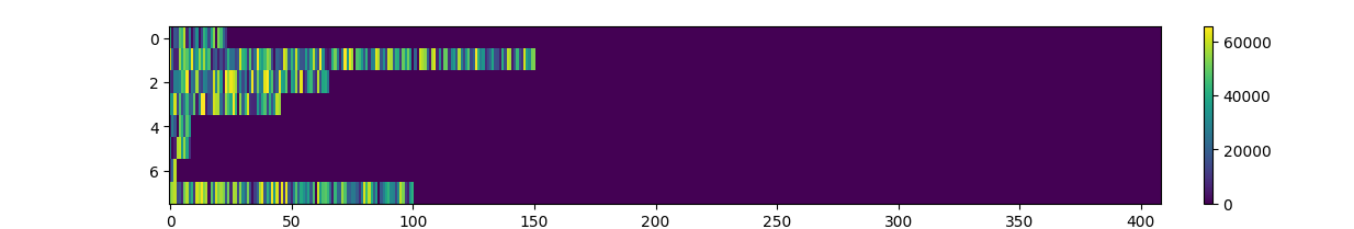
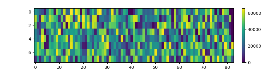
Here, we have a heatmap that shows the first batch of 8 reviews. Every row is a document, and all documents have now been padded to 409 tokens as part of the batching. Here, each color represents a token at a specific point in a review. The colors go up to 60000 or so, as that is the largest vocabulary index present in this batch. Now is a good time to remind ourselves - the tokens that make up a review were randomly generated. This means that any time the same color appears twice, that means there is a duplicate token. One can’t help but notice the massive purple section at the end of every single row. That’s all just padding.

As was discussed earlier, the first step of the model’s forward pass is a multiplication with a matrix of size $\mathbb{R}^{4096 \times 4096}$. Each of the eight rows in the above image will be a $\mathbb{R}^{409 \times 4096}$ matrix when entering this operation. All the values in the resulting $\mathbb{R}^{409 \times 4096}$ matrix will be calculated. For the first review, only 24 of the rows are ever used. For the 7th review, only 9 of the rows are ever used. The rest of the tokens are just padding, after all, and will be ignored. We could’ve passed these through as $\mathbb{R}^{24 \times 4096}$ and $\mathbb{R}^{9 \times 4096}$ matrices, but have decided to turn them into these mammoths for the sake of batching. This repeats for all intermediate steps during the forward pass, as the reviews make their way to the last linear layer with their dimensionalities intact.

This process gets repeated over and over for all batches, with us either discarding or masking out all of the values that get calculated for the padding tokens. Thinking for a moment about how matrix multiplications happen inside a GPU, there is a limited amount raw computations that can be performed in any given timeframe. When we process a batch like this, we are saturating that capacity with garbage calculations whose results will get thrown out as soon as they finish. Here is the heatmap for the entire dataset:

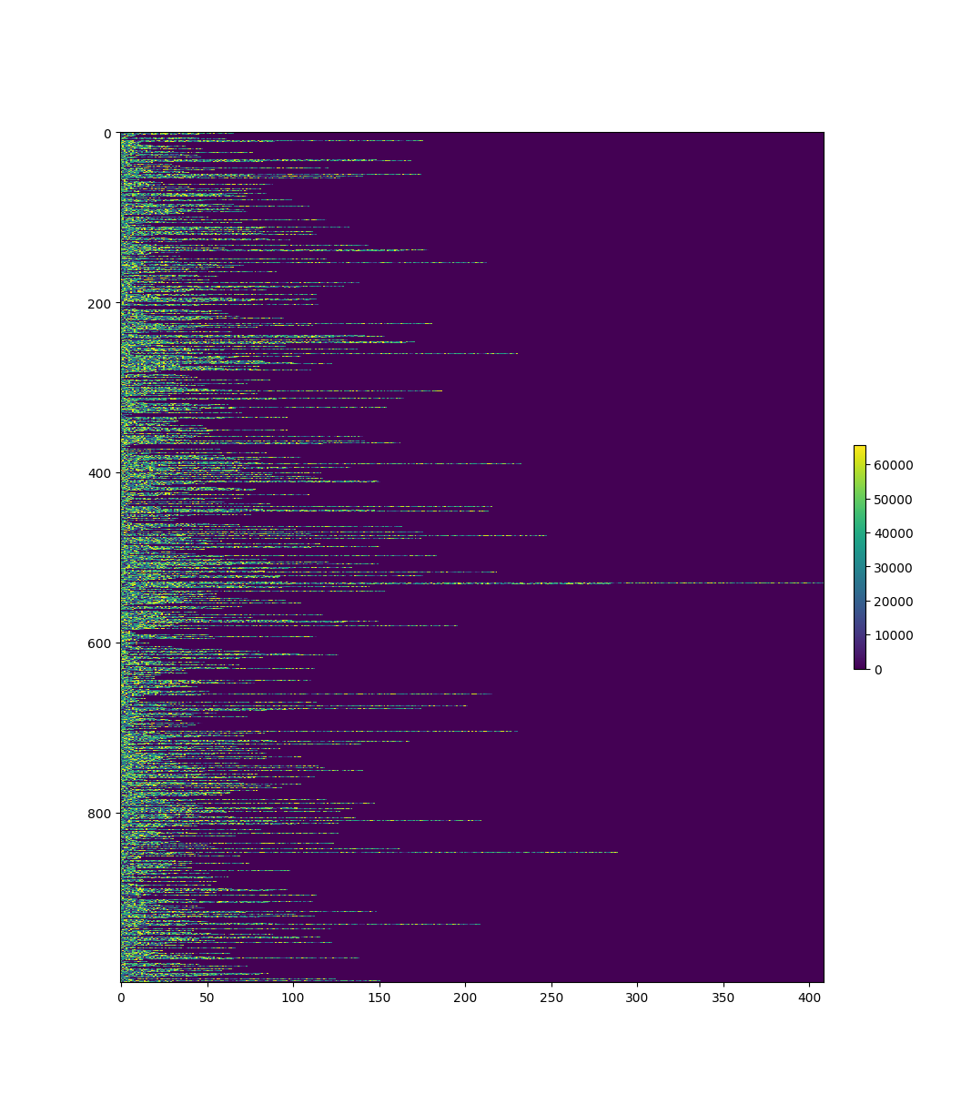
We can see that this is not an isolated indicent. It almost doesn’t even matter where you slice your batch of 8 reviews, you’re mostly just processing garbage. There’s exactly one batch where there is any sort of justification for this level of padding, and that’s the one with the longest review.

Getting industrious

Here’s an idea that probably comes to mind: Let’s first choose our 8 reviews and place them in a batch, and then pad according to the maximum length in that batch. Our implementation only changes a tiny bit as we shift the padding down by two lines, applying it only after creating the batch:

def batch(model: WhateverModel, documents: list[list[int]]):
    sentiments = []

    for batch_start in range(0, num_docs, batch_size):
        batch = documents[batch_start : batch_start + batch_size]
        batch = pad_documents(model, batch)

        # Forward pass of the model
        sentiments.extend(model.forward(batch))

    return sentiments

The padding is now done inside a loop instead of all at once, but that process is effectively instant. More importantly, look at how much the first batch’s heatmap improves:

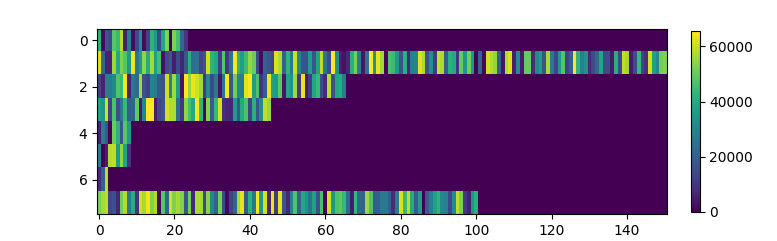
Now we’re cooking. The massive wave of purple at the end of each review is gone, and we are only processing what we need to process. Sure, we’re still calculating some garbage, but that’s just the price you pay for batch processing. After all, we can’t do any less padding, as we have padded to the length of the shortest review in the batch. The only way we could do better would be to reduce the length of the shortest review in the batch.

Hardly working

Here’s what you should actually do: simply sort your reviews based on length, and then pad each batch separately. In terms of code, we add one line before the loop:

def batch(model: WhateverModel, documents: list[list[int]]):
    sentiments = []

    documents.sort(key=lambda x: len(x))
    for batch_start in range(0, num_docs, batch_size):
        batch = documents[batch_start : batch_start + batch_size]
        batch = pad_documents(model, batch)

        # Forward pass of the model
        sentiments.extend(model.forward(batch))

    return sentiments

It doesn’t get any simpler than this.

We group reviews based on their length, and then place reviews from the same group to the same batches. After all, the downside in the previous approach was that the batch contained reviews of differing lengths due to chance. Don’t count on your luck to segment the reviews into perfect batches, it’s not going to happen.

I won’t show you the first batch, as it’s just a matrix of 8 scalars (ie. 1-word reviews). Instead, here’s the 101st batch, containing the reviews indexed 800 to 808:

There’s barely any padding, even as we approach the end of our dataset, where there are less reviews and length differences between reviews become more pronounced.

So what?

So does any of this matter? Is this really all that useful? Are the additional computations introduced by the sorting even worth it? Here are the results on a RTX 4080 SUPER:

Batching	Time taken (seconds)
Birdbrained	58.681
Industrious	17.579
Clever	8.406

Quite the jump, and remember: we are performing exact inference, producing the same output. There are no stochastic approximations or unfounded assumptions here, the results are unchanged. And yet, the runtime drops sevenfold.

This can also be motivated in a more visual sense through an Area Under Curve (AUC):

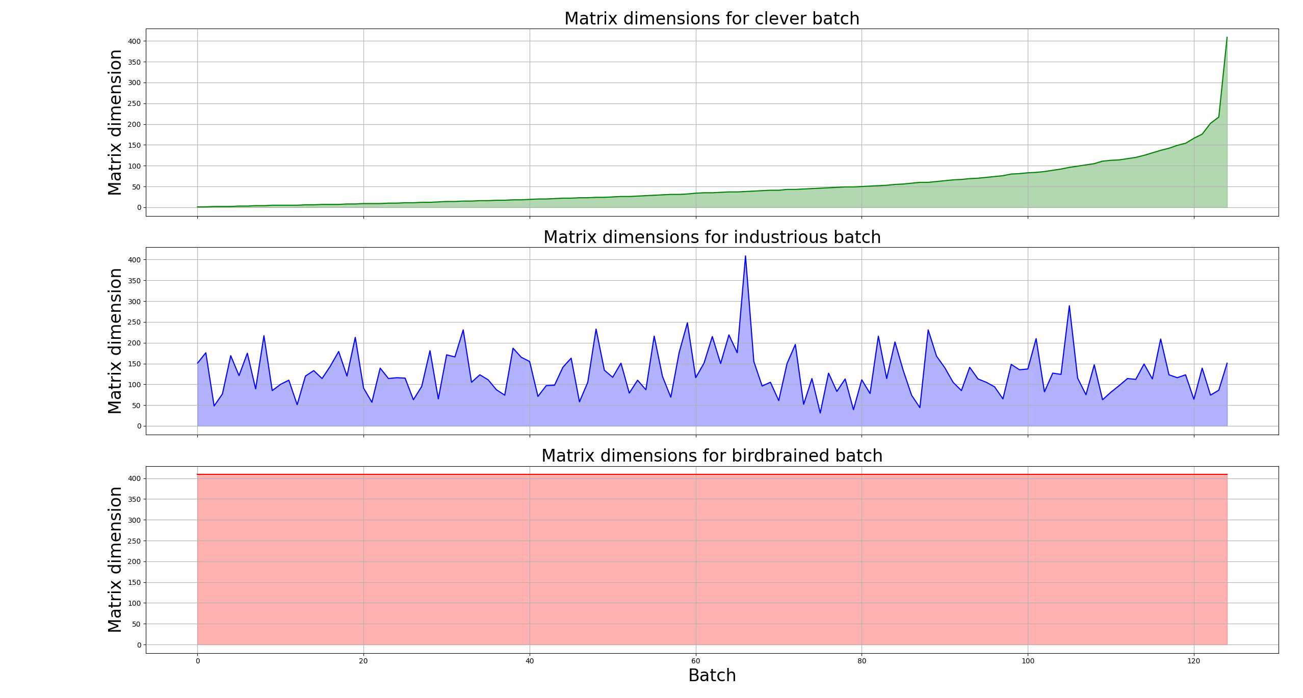
Here, we have plotted the first dimensions of the matrices being passed through the model in each batch. This is to say, we are plotting the length that each review is padded to in each batch. As this value defines the dimensionality of the matrices being multiplied during the forward pass, it is a good litmus test for computational complexity. The larger the colored area, the more computation is required. Let’s place these graphs on top of each other:

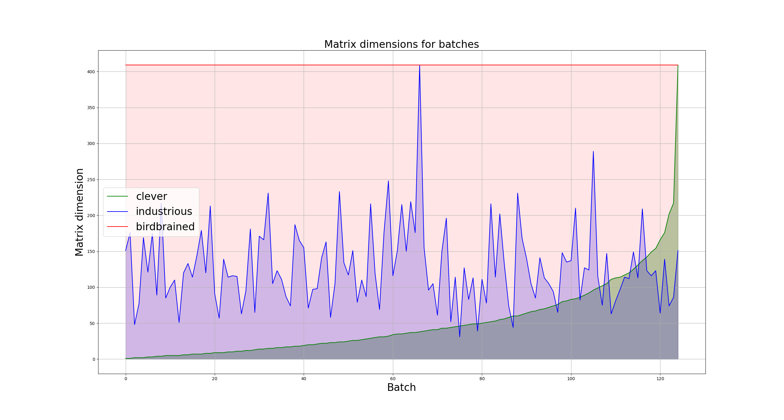
It becomes clear just how much better we end up doing by changing two lines of code.

Honing the blade

There are also further optimizations that could be performed. As mentioned, when using the birdbrained batching approach, the maximum batch size possible with my GPU is 8. This is also true for the later two, as we still need to process the batch that contains the longest review sooner or later. At that point, we will need to allocate memory for the full $\mathbb{R}^{\text{batch size} \times 409 \times 4096}$ matrix anyways. And yes, with a constant batch size there’s no getting away from this fact. However, if we allow the batch size to change dynamically, we can actually squeeze out just a bit more perforamance yet.

Instead of setting a batch size limit, let’s set both a token limit and a length delta limit between the reviews within a single batch. Now, we add reviews to our batch until one of those limits is reached, and then process the batch. The first limit makes sure our GPU doesn’t run out of global memory, and the second makes sure we don’t start processing too much garbage again. This gets a bit more involved than the previous approaches, but it drops the runtime down to 7.306 seconds.

def batch(model: WhateverModel, documents: list[list[int]]):
    sentiments = []
    documents.sort(key=lambda x: len(x))

    max_tokens_per_batch = 21000
    max_length_diff_within_batch = 8

    batch_start = 0
    curr_index = 0
    while curr_index < num_docs:
        curr_batch_tokens = 0
        curr_batch_min_length = len(documents[batch_start])

        batch = []
        while curr_index < num_docs:
            next_doc_len = len(documents[curr_index])
            if (
                next_doc_len - curr_batch_min_length > max_length_diff_within_batch
                or curr_batch_tokens + next_doc_len >= max_tokens_per_batch
            ):
                break

            curr_batch_tokens += len(documents[curr_index])
            curr_index += 1

        batch = documents[batch_start:curr_index]
        batch = pad_documents(model, batch)

        # Forward pass of the model
        sentiments.extend(model.forward(batch))

        batch_start = curr_index

    return sentiments

Wrapping up

I’m hesitant to call batching a necessary evil, as there really is nothing nefarious about it. This is not to say that I think it’s trivial, far from it. There’s always going to be trade-offs and it’s never going to be quite perfect as long as your data stream is not 100% consistent and predictable. It’s part of every ML model training cycle and effectively every deployment of said models, so it’s important to figure it out. But the most important thing is that if you are batching data that can’t be concatenated directly into a tensor, don’t just pad them naively to make the problem go away. Think about it for just a bit, or you’ll end up doing birdbrain batching.

The code for these experiments can be found in this Github repository.