When you should not use a GPU to run a machine learning model
A general consensus even among some machine learning practicioners appears to be that you should always use a GPU when running inference. Even in small embedded devices, you should just throw on a Jetson Nano and call it a day. It has a GPU after all, something you should always have when using a machine learning model. Don’t get me wrong, there is some truth to this. A GPU is often the only sensible choice in the current landscape of models with billions of parameters that are applied generally to problems without any task-specific training. It has also gotten a lot easier to just slap on a GPU or to call an API that then uses one remotely, there’s no denying that. However, to say that you should always reach for a GPU when running inference is not the full picture. This post is about explaining one such situation where you shouldn’t use a GPU, and distilling some rules about when this may occur more generally.
Definitions
Model: Some machine learning model. Can be assumed to mean a bog-standard feed-forward neural network with some amount of linear layers joined by ordinary nonlinear functions.
Datapoint: The input to the model. Can be assumed to mean a vector of some dimensionality.
Batch: A set of datapoints that will be passed through the model in parallel. This is done to improve performance over the datapoints being passed through sequentially. For the reasons why this is, see here.
Ply: When one player has taken an action in a two-player game. This is in contrast to the more ambiguous term move, which can also mean when both players have taken an action.
A pernicious shortcoming
When running inference, GPUs can only run operations on data that has been transfered over the memory bus from system memory to the GPU’s internal memory. The model parameters are usually not important here, as we can just keep them in the GPU’s internal memory for as long as we expect to use the model. However, the same cannot be said for the datapoints. Each non-trivial datapoint is unique, meaning we are granted no such luxury. Imagine a scenario where you transfer a small batch of data to the GPU’s memory, utilize it only for a handful of operations, and then inevitably have to transfer the results back over to system memory. Suddenly, this overhead from data transfer and communication between the CPU and GPU starts to matter, and GPUs start to get clumsy. This idea could be visualized like this:
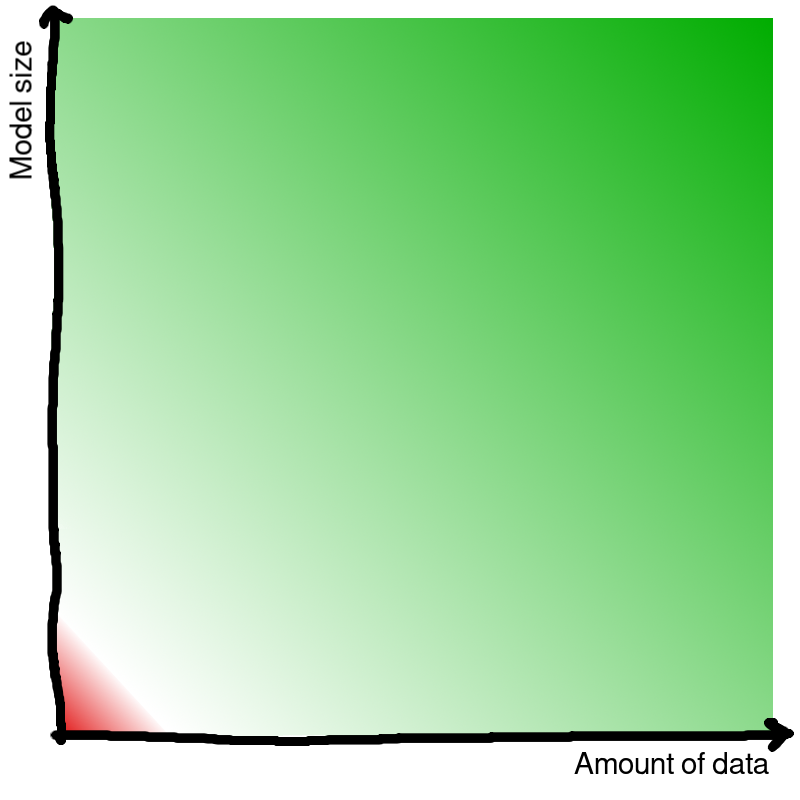
An important note is that if you’re facing only one of these two factors, it can often be offset by the other. Does you batch only contain a single datapoint? Well, if your model is 8 billion parameters, you’re still better off using a GPU. There is still a mountain of matrix multiplications that could be performed in parallel due to the size of the model’s weight matrices. Conversely, do you have a model that has only a few thousand parameters? Alright, but does your batch also contain $100 000$ datapoints? Because if it does, you’re still better off delegating that workload to the GPU. The number of matrix multiplications that could be performed in parallel starts to compound from the number of individual datapoints you will be passing through this model.
A completely sensible reaction to this statement would be “Who cares?”. We’re running a small model and only passing through a handful of datapoints, so the amount of time taken will probably not be long anyways. So why does it matter if the GPU is going to be a bit slow?
Setting the stage
Think of any two-player, deterministic, zero-sum, perfect-information, non-cooperative game. This is to say chess, checkers, go, connect four, tic-tac-toe… In solving such games computationally, the tried-and-tested method is the minimax algoritm (or it’s mathematically equivalent negamax algorithm).
In minimax, you come up with some measure of which side is winning, and then you assume that one player is maximizing this value and the other side is minimizing it. Let’s call this the evaluation of the position. You assume that both players are going to play optimally according to this evaluation, and start exploring the different legal moves present in the position. If you were to choose a move for yourself, then one for you opponent, another move for yourself, and so on, you would form a chain of $n$ moves. These $n$ moves would result in $n - 1$ intermediate positions and one resulting position. Let’s call these chains of moves lines. Combining all possible lines would form a game tree; a graph representing the possible game states moving forward. Here is an example of what a (partial) game tree for tic-tac-toe could look like:

A naive implementation of minimax would proceed as follows:
- Form the game tree up (or down?) to some maximum depth and evaluate the final positions.
- Propagate the evaluations of the final positions up the tree by alternating between maximization and minimization at each depth.
- Now that these evaluations also reflect the opponent’s best attempts at countering your moves, just choose the immediate move that has the highest evaluation in the resulting tree.
What’s fantastic about this approach is that you can pass all the final positions through the model in one batch (VRAM permitting) and get their evaluations rather efficiently.
To turn this into negamax instead, you just call the same evaluation function with $(-beta, -alpha)$ instead of $(alpha, beta)$ while working your way down the tree, and then negate the value returned. This way you can always just maximize inside the evaluation function itself. It’s nothing more than a code simplifying manoeuvre, a cosmetic reformulation relying on the zero-sum assumption of the game.
As you can guess, this doesn’t work for anything much more complicated than tic-tac-toe. We’re going to be focusing on chess and using Stockfish as an example going forward. It has been the strongest chess engine around for a decade and counting, and it uses negamax at its core.
In a game like chess, if you start evaluating the positions resulting from each legal move, you won’t get far. Here’s the sequence counting the number of unique chess positions after $n$ plies.
\[20 \\ 400 \\ 8902 \\ 197281 \\ 4865609 \\ 119060324 \\ 3195901860 \\ 84998978956 \\ 2439530234167 \\ 69352859712417 \\ 2097651003696806 \\ 62854969236701747 \\ 1981066775000396239 \\ 61885021521585529237 \\ 2015099950053364471960 \\\]If you wanted to run that algorithm with a depth of 10 plies from the starting position, there would be 69,352,859,712,417 unique positions for you to evaluate at the bottom of the tree. This is assuming that you’re using a transposition table to recognize duplicate positions, allowing you to omit re-evaluating the many positions that occur in multiple lines. In the end, this would only allow you to see 10 plies ahead, and things would only get more ridiculous from here. This is because chess has a relatively high branching factor, meaning there are many possible moves in each position.
So a problem clearly arises from this approach: How to know which lines are worth inspecting without actually inspecting them?
This simple problem has inspired enough textbooks and academic articles to fill a library, but here are some examples from the aforementioned Stockfish chess engine. All code snippets have been taken from the current version of search.cpp and slightly modified for readability.
- Late Move Reductions, or Spend less time thinking about moves that don’t seem too appealing on first glance. If we’re proven wrong by the resulting shallow search, continue with the proper search instead.
// Here, r is a "reduction" variable, which is higher
// when a move doesn't seem like a great candidate for
// a deeper analysis.
if (depth >= 2 && moveCount > 1)
{
    Depth d = std::max(1, std::min(newDepth - r / 1024, newDepth + 2)) + PvNode;
    (...)
    value = -search<NonPV>(pos, ss + 1, -(alpha + 1), -alpha, d, true);
    (...)

    // Do a full-depth search when reduced LMR search fails high
    if (value > alpha)
    {
        (...)
    }
}- Static Exchange Evaluation, or “If a move initiates a bunch of trades on that square which leave you down material in the end, ignore it.”
// Do not search moves with bad enough SEE values
if (!pos.see_ge(move, -80))
continue;- Futility pruning, or “If we look at a move through rose-tinted glasses and it still looks hopeless, just ignore it.”
Value futilityValue = ss->staticEval + 42 + 161 * !bestMove + 127 * lmrDepth
                    + 85 * (ss->staticEval > alpha);
if (!ss->inCheck && lmrDepth < 13 && futilityValue <= alpha)
{
    (...)
    continue;
}
One could go on: ProbCut, Singular Extensions, Internal Iterative Reductions, Multi-cut pruning, Null Move Pruning… However, the one theme that shadows over the entire searching process is hinted at in the third code snippet: Alpha-Beta pruning.
At the core of alpha-beta pruning is a simple question: Knowing the other lines we have already looked at, could this one ever be worth investigating further?
If a line is so bad compared to the alternatives that we would never allow it, there’s no need to look further. Such a line is said to Fail low.
Conversely, if a line is so good compared to the alternatives that the opponent would never allow it, there’s also no need to look further. Such a line is said to Fail high.
All other lines are fair game. Alpha-Beta pruning has a nice property in that it’s not necessarily a heuristic. This is to say, it’s not some practical shortcut that produces “good enough” results without taking into account all related information. If the evaluations are accurate, it only makes us ignore lines that could not affect the our decision. Of course, the evaluations used in Stockfish are not based on perfect information, so this isn’t always true in our example.
Before continuing, there is one term that needs to be explained: quiescence search. When the search depth is reached, an engine is going to stop searching further down the game tree. The obvious thing to do would be to just return the static evaluation of the position. However, if the position is not quiet but has tactical moves instead, this static evaluation will have a hard time conveying the position’s tactical intricacies. This could lead to an overly high evaluation for a position that is tactically losing, or an overly low evaluation for a position that is tactically winning. Therefore, engines have adopted quiescence search, which continues the search until the position becomes quiet again by doing a mini-search over all tactical moves. We will see why this explanation was necessary in just a bit.
With that out of the way, you can see alpha-beta pruning in action when Stockfish decides what to do with a position once it has been evaluated:
// bestValue = -infinity
(*loop over all legal moves*) {
    // get the value of the resulting position with some depth...

    if (value > bestValue)
    {
        bestValue = value;

        if (value > alpha)
        {
            bestMove = move;

            if (value >= beta)
            {
                (...)
                break;
            }
        }
    }
}
One of the moves in the position leads to a situation that is so good for us, that it beats $beta$. Here, $beta$ stands for the best position that the opponent can force in some other line. Therefore, you have to assume that the opponent would never grant you the opportunity to make this move, meaning they won’t allow the preceding position. As such, the search exits right away, and this line fails high.
Similarly, here is what happens immediately after a given position’s static evaluation has been calculated by passing it through the evaluation model (a simple neural network):
if (eval < alpha - 485 - 281 * depth * depth)
    return qsearch<NonPV>(pos, ss, alpha, beta);
If the position is much worse than alpha (the best position we know we can get by playing another line), then we probably won’t find anything better by digging deeper. Here, qsearch stands for quiescence search. We are immediately ending the search into this line, but doing so in a sensible manner. Therefore, we simply dot our i’s and cross our t’s by running quiescence search, and then return the position’s evaluation. This line has now failed low.
Bringing it all together
So in this scenario, we first evaluate the position with the model, and then decide how we should proceed. Once the model’s evaluation has been calculated, we might:
- End the investigation into this line completely.
- Search some, but not all, of the position’s continuations further.
- Continue the investigation into this line.
- End an investigation into a completely different line that is being evaluated in parallel.
- Decide to not investigate a line in the future that may or may not be related to this one.
- Restart the investigation into the position leading up to this one, even though it was initially discarded.
And so on. It all depends on how this position is evaluated.
Hopefully the reason for this tangent is starting to become clear. In running these kinds of algorithms, the model is small and we are only passing a small batch through it. In fact, each of our batches only contains one datapoint. Furthermore, the model’s result very conceretely affects, which batches will be passed through the model in the future. There is effectively an infinite amount of work we could be doing, but we can’t reasonably do it all, most of it is pointless and the only way to find useful work relies on incremental exploration. This is exactly the type of machine learning inference where GPUs stumble, and it happens every time someone plays against a chess engine.
What to do?
Let’s think about solutions for a moment instead of just problems. We still want to run linear algebra operations, but we would like to do away with the memory transfer from RAM to VRAM and the delay caused by communication between the CPU and the GPU. Well, how slow would it be to just use the CPU instead? Although the original x86 instruction set had no notion of vectorized instructions that could be suitable for a task like this, the instruction set has been maimed and mutilated for 50 years now. As it turns out, this process has left us with some useful tools to work with.
If you’re interested in the practical side of using these tools, called SIMD instructions, you can check out this post. For our purposes, it is sufficient to know that modern CPUs can be made quite performant at the types of operations required by neural networks. In fact, once you factor in the data transfer overhead and assume a small enough model, CPUs might start to look like a better option.
Putting some meat on the bone
Alright, I’ve laid out the scenario where I claim that using a CPU could beat out a GPU. It’s just words, though, and doesn’t do any good unless I can prove it. Better yet, I should be able to put at least some real numbers behind my words.
For this reason, I’ve benchmarked the process of calculating a GEneral Matrix Multiplication (GEMM), ie. $C = \alpha AB + \beta C$, at different dimensionalities. The experiment is using $\alpha = \beta = 1$ and three square matrices with the same dimensionality. The implementations are simple C++ functions that get three pointers to arrays of data, and the timer is started immediately. As such, we’re counting memory allocation, data transfer and freeing of the allocated memory for the GPU on each iteration. A GEMM is exactly what happens, when we have a matrix size of $\theta$ and
- We have a batch size of $\theta$ datapoints.
- Our feature vectors are $\theta$ values wide.
- We’re passing this data through a linear layer whose width is $\theta$.
- The linear layer is using a bias.
As such, this operation should be an accurate proxy for batched machine learning inference.
The CPU implementation is using OpenBLAS (0.3.30) through the cblas.h header with an AMD Ryzen 9 7900X.
For the GPU, I’m using cuBLAS kernels from CUDA toolkit (13.0.2) through the cublas_v2.h header with a RTX 4080 SUPER.
Both of these implementations should be getting fairly close to the optimum performance for their respective hardware.
Let’s get to the results. The X-axis shows the shared dimensionality of the matrices being used as operands, ie. our $\theta$ from above. The matrices are all initialized with random 32-bit floating point numbers between 0 and 1, and the calculations at each size are run 100 times to reduce randomness. Afterwards, we take the median (not mean) of the wall-clock times in seconds, and plot them on the Y-axis. Blue line is the CPU and orange line is the GPU:
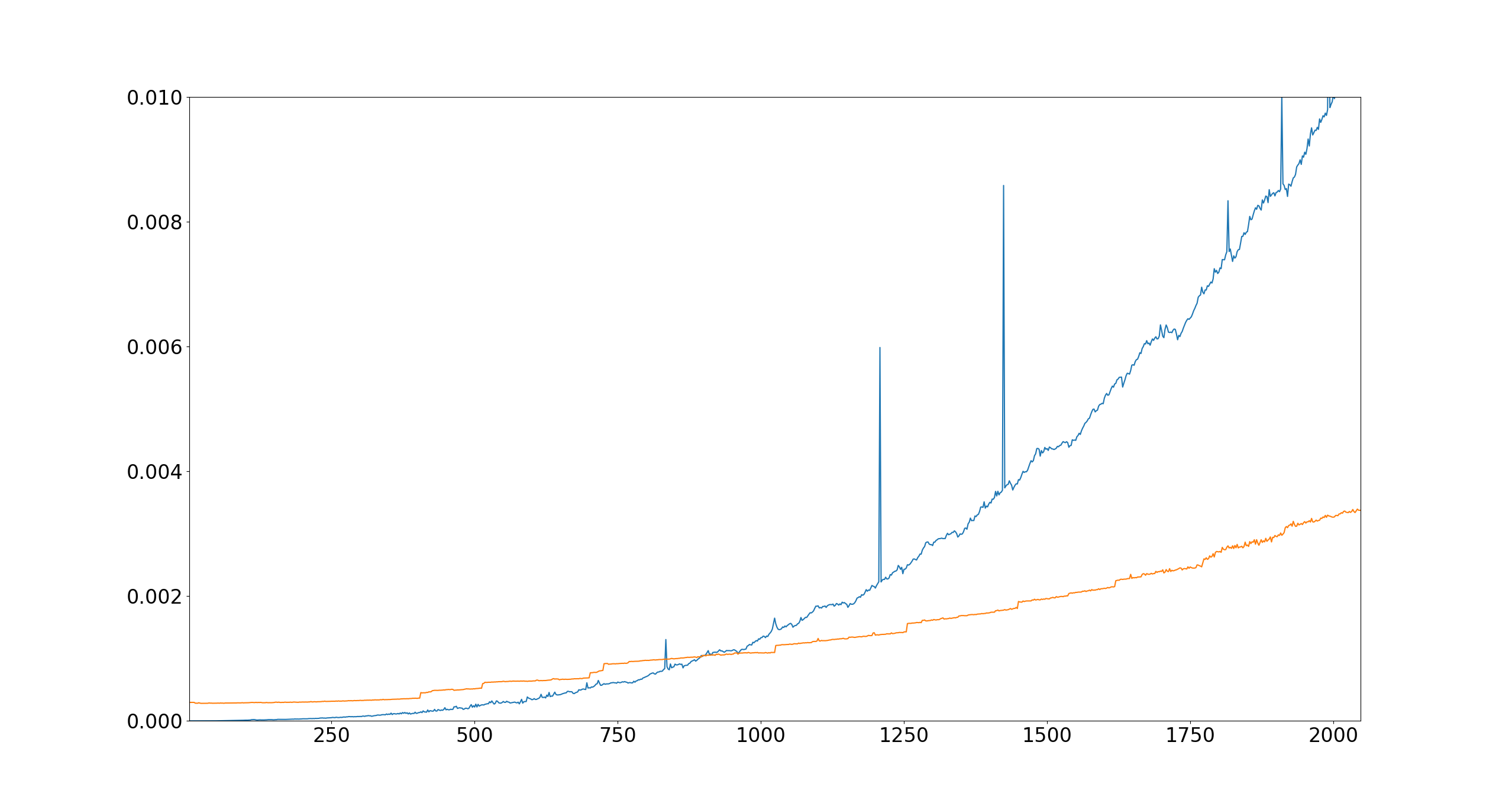
Looking at the data, there are a couple of peculiar jumps for the CPU. I’d assume these are the result of random noise due other system processes causing interrupts and like, as we are benchmarking an operation with a very short wall-clock time. All in all, a very clear trend for the CPU.
For the GPU, even the smallest operation takes around $0.0003$ seconds. The runtime remains stable for a long time in the start, which would suggest that this minimum runtime is imposed by the communication overhead and kernel launch latency, and not the data transfer. Curiously, if we look at the GPU data as a whole, it looks like a sequence of step functions with relatively linear increases between them. Here’s my theory as to why this happens:
The gradual increase in runtime between the steps is from data transfer overhead. Our computation is memory bound, so incrementally more data means an incrementally longer runtime. Then, there are occasional big steps. When a big step happens, it indicates that some computational complexity threshold has been reached. These steps seem to be split into two parts: steps before the size 1024x1024, and those after it. The fact that this split happens exactly at a power of 2 is a strong clue.
First, the steps after this point happen rougly every 200 dimensions. I have to admit that the reason for this exact number is a mystery to me. The GPU operates in tiles with a set size, like 128x128, which would mean that the runtime should jump every time a multiple of this tile size is reached. This is because between these multiples, some tiles have padding in them which could be replaced with meaningful data for free as the matrix grows. Once all tiles are full, there has to be a new tile added to the computation, which means many additional calculations (most of which are pointless in the beginning). However, I don’t think the cuBLAS kernel would be using a tile size of 200, and the distances are not exactly the same each time. If you think you know the answer, I’d love to hear your theory.
The steps before this point seem more erratic. This might be because cuBLAS is switching between kernels that are optimized for different sizes. The same kernel might be used from 1024x1024 onwards, which would explain the relative stability afterwards. Again, not sure on this one, but the trend seems to be clear and fairly consistent.
In any case, there are definitely matrix sizes where I’d take the CPU on any day of the week. In fact, any matrix size below 850 or so seems to be a clear win for the CPU. This amounts to roughly $2 \cdot 850^3 = 1.3$ billion floating point operations.
Of course, when the number of operations grows past a certain point, the GPU starts to slowly mop the floor with the CPU. If we kept going for a while, the line for the GPU would start to look horizontal compared to the CPU. Furthermore, if we dropped the precision down to 16-bit, 8-bit or especially 4-bit floating point values, the GPU would start utilizing tensor cores and we would be transfering much less data. This should make the GPU perform better. All of this is to be expected, though, as this would be the CPU fighting on the GPU’s home field - a place that it was never really designed for. The opposite would be true if we switched to integers, so these speculations are not meaningful on their own.
Some may be wondering how much the results would change if ignored the GPU’s operations related to memory allocations and data transfer. In the below plot, all memory on the GPU is pre-allocated, data is pre-transferred, and no results are brought back to RAM while the timer is running:
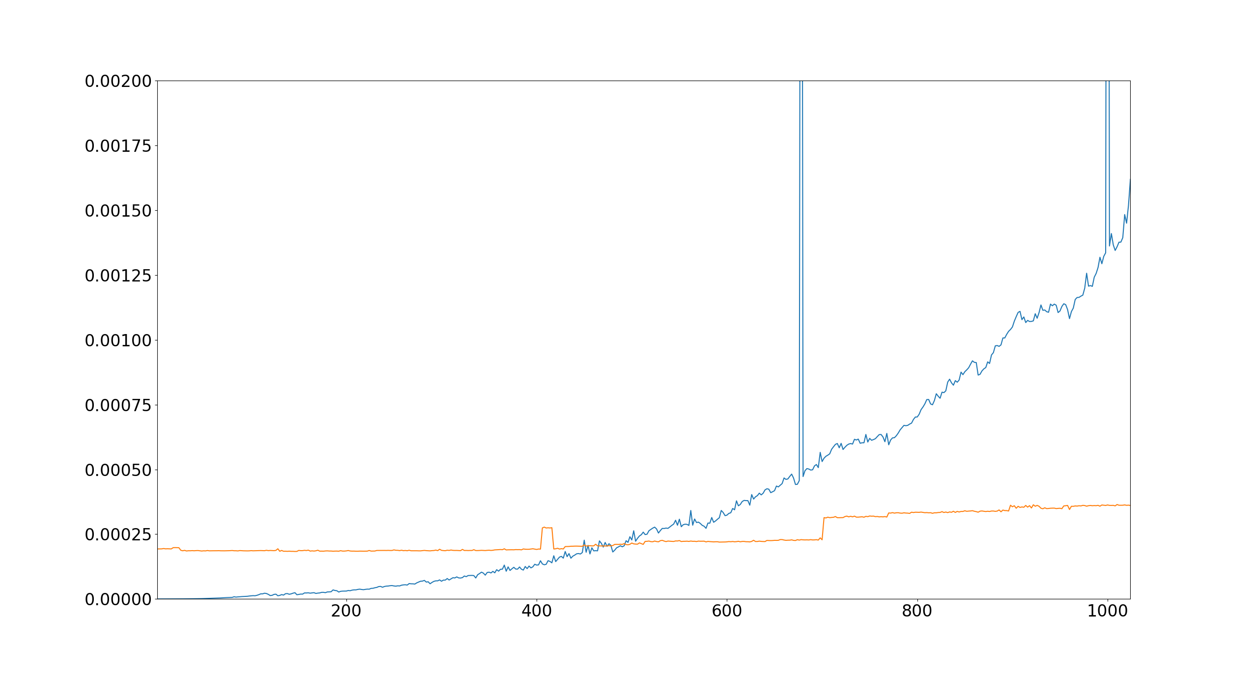
Do with this data as you will, as long as you don’t take it as gospel. I’m contempt in claiming that I’ve proven my point.
Closing thoughts
This example of a two-player game being solved with minimax is far from the only instance where GPUs begin to falter. Any scenario where small batches of data must be passed through a small model sequentially will arrive at the same dilemma. Like any performance consideration, there is no textbook from which you could just look up the solution to your specific problem. You have to try many options, and then choose the one that worked the best. The skill doesn’t lie in trying to guess the right answer on the first try, but in how many different ideas you can come up with in total.
Sources
https://en.wikipedia.org/wiki/Game_tree#/media/File:Tic-tac-toe-game-tree.svg
https://oeis.org/A048987
Notes
The code used for comparing the CPU and GPU runtimes can be found here.
If you wanted to be precise you would say that Stockfish uses a NNUE, an Efficiently Updatable Neural Network. This just means that Stockfish formulates the inputs to the neural network in a way where most of the calculations in the first layer do not need to be performed again after a move is made. Subsequently, the number of calculations required to evaluate a position is even smaller than the model size would indicate, further exacerbating the issues faced by GPUs.
The scenario outlined in this post is of course not the only one where GPUs are the wrong tool for the job. As pointed out by the initial definitions, I’m excluding all machine learning models that don’t make extensive use of matrix multiplications. A GPU is not designed for such workloads, and is clearly going to do a horrible job.
There are also scenarios where GPUs are not fit to handle large neural networks, even when using a large batch size. For instance, if a model’s size stems from having a large number of layers whose weight matrices are all exceedingly small. The reasons for building such a network are beyond my understanding, but in this case you might actually not be able to utilize the parallelism of the GPU; all the operations are small and have to be run sequentially. Additionally, let’s say a model requires some exotic data type that is not supported by standard GPU kernels. There is little you can do to make this work on a GPU, if anything. I would, however, claim that the scenario outlined in this post is the most common occurrence of CPUs beating out GPUs in machine learning inference, and not by a narrow margin.